Contents
I. Introduction 1
II. General Operation 2
A. Stepping through Modeig/II 2
B. Commands Menu 4
1. C - Commands 4
2. E - Edit 4
3. H - Help 4
4. N - New 4
5. Q - Quit 5
6. V - View 5
7. X - eXit 5
III. Input File Cards 6
IV. Structure 7
A. Direct Layer Input 7
B. Indirect Layer Input 8
C. Graded Layers 8
D. Multiple Quantum Wells 9
E. Auto Quantum Well Width Calculation (GaAs) 9
F. Symmetric Grinsch Structure 10
G. Asymmetric Grinsch Structure 10
V. Near and Far Field Calculations 12
VI. Confinement Factor Calculations (Gamma) 13
VII. Looping 14
A. Low-level (X looping) 14
B. High-level (Z looping) 15
C. Initial Guess Generation 16
D. Wavelength vs. Quantum Well Width 17
E. Multiple Output File Generation 17
VIII. Output 18
A. Output File General Information 18
B. Dbase File 19
C. Layers File 21
D. Output File 21
E. Nfield File 21
F. Ffield File 22
Variable Glossary 23
CASE PARAMETERS 24
MODCON PARAMETERS 30
STRUCT PARAMETERS 33
LAYER PARAMETERS 34
GAMOUT PARAMETERS 35
LOOPX PARAMETERS 36
LOOPZ PARAMETERS 37
OUTPUT PARAMETERS 38
Appendices 39
Appendix 1 40
Appendix 2 41
Appendix 3 42
Appendix 4 43
Appendix1_dbase 44
Appendix1_layers 45
Appendix1_output 46
Appendix1_nfield 53
Appendix1_ffield 54
Pictures 58
PICTURE 1 59
PICTURE 2 60
Error Messages 61
File system errors 61
Runtine error codes 62
I. Introduction
The Modeig/II manual is designed to be a reference guide to using the Modeig/II program on the Macintosh. Specific details about the calculations performed can be found in :
EE Technical Report No. 206
December, 1977
by:
Robert B. Smith
Gordon L. Mitchell
Additional information can be found in:
Modeig Users Manual
February 13, 1987
by:
V.J. Masin
G.A. Evans
Recommended Hardware:
Apple Macintosh II
Recommended Software:
text editor: QUED-M v2.07 or later
graphics: CRICKET GRAPH v1.3 or later
This manual uses the following notation:
< > - characters in between the brackets should be typed on the keyboard
! - comment separator, everything to the right of the exclamation point is a descriptive comment
II. General Operation
A. Stepping through Modeig/II
To run Modeig/II double-click on the 'Modeig/II apl' icon. The Modeig/II header and revision date will be displayed on the screen along with the prompt for the input filename. Type in the name of the input file to continue with the Modeig/II program or type a command from the commands menu (see II. B). The input filename can be up to 31 characters long (not including the directory path) and can contain all of the standard Macintosh filename characters except for a blank space. The input file should be a text file similar to the files shown in the Appendices. The file does not have to reside on the same disk as the Modeig/II application, adding the directory path as a prefix to the input filename will cause Modeig/II to search the specified disk for the input file.
HD20:MODELING:inputfile
In the above response 'HD20:MODELING:' is the directory path and 'inputfile' is the input filename. This response would cause Modeig/II to search the folder named 'MODELING' on the disk 'HD20' for the file 'inputfile'.
The next prompt is for the output filename. Pressing the <return> key will default the output filename to the same name as the input file and the file storage location to the same disk where the input file resides. Suffixes are appended to the output filename to indicate the type of data in the file ('_layer','_output','_dbase',...).
Entering a different name for the output filename will cause Modeig/II to store the data files using the filename and directory path entered. If no directory path is given, the disk where the Modeig/II application resides will be used.
Response Data stored to:
<return> : HD20:MODELING:inputfile_sfx
DISK2:NEWFOLDER:inputfile : DISK2:NEWFOLDER:inputfile_sfx
CAUTION:
Modeig/II will attempt to store all of the output data files to the disk specified. If large amounts of output is to be generated, the '_output' file is turned on, it is a good idea to specify the hard disk as the directory path for the output to avoid a 'DISK IS FULL' error during execution of Modeig/II. If a 'DISK IS FULL' error is encountered, the error message will be displayed along with a prompt to type the <return> key. Upon entering the <return> key the Modeig/II program will quit and control will return to the Macintosh Finder.
After receiving the input and output filenames Modeig/II will attempt to read the input file. If Modeig/II cannot find the input file on the disk specified an 'INPUT FILE NOT FOUND' error message will result along with a warning bell. Modeig/II will then prompt for another input filename.
If the input file is found, Modeig/II will attempt to read the input displaying each line as it is processed. If Modeig/II finds an illegal input card or parameter an error message will result specifying the card or parameter which caused the error and a prompt to continue will be displayed.
After successfully reading an input file Modeig/II will prompt to continue. Entering a <return> will continue with the Modeig/II program, a <Q> will quit the program, and a <V> will display (view) the layer information generated from the input file. All the commands from the commands menu are available at this time.
Continuing with the program, Modeig/II will display a listing of the output files created and will then start the calculations. The output data will be displayed on the screen in columnar format with the loop variables listed first in order of looping.
Execution of the calculations can be stopped at any time by typing < command . >. This break will cause Modeig/II to prompt for a <return> to quit.
Upon completion of the calculations Modeig/II will prompt for 'Another case?'. A <return> or <N> response will quit Modeig/II and return to the Macintosh Finder. A <Y> response will cause Modeig/II to prompt for another input filename and the whole input process starts again.
The output files generated by Modeig/II can be viewed using an editor. The output files can then be printed using the editor's standard 'PRINT' routine.
The '_dbase', '_nfield', and '_ffield' output files are in tab delimited columnar format with column headers and a leading asterisk. This format is used for input files by many graphics software packages so graphical outputs are easily obtained.
B. Commands Menu
The Commands menu is a listing of all the command modes available while accessing the input file. The following commands are available:
C - Commands ! lists the commands menu
E - Edit ! allows line appending to input file
H - Help ! displays users manual on screen
N - New ! allows creation of new input file
Q - Quit ! quits the Modeig/II program
V - View ! views the layer info for the structure
X - eXit ! exits the current command mode
1. C - Commands
The <C> command lists the commands menu to the screen.
2. E - Edit
The <E> command puts Modeig/II in the Edit mode. The editor allows changes to be made to the input file while running the Modeig/II program. If an input file has not been read in by Modeig/II the editor will prompt for the name of an input file, if the entered filename does not exist, a new input file will be created.
The editor will display a '?' prompt when layer information can be input. Any text entered at the '?' prompt will be appended to the end of the input file selected, this feature allows on-line changes to be made to the input structure. Entering an <X> will exit the editor.
3. H - Help
The <H> command puts Modeig/II into the Help mode. This mode displays the users manual on the screen one page at a time, entering <return> displays the next page, an <X> exits Help mode.
4. N - New
The <N> command is used to create a new input file. After prompting for a new filename Modeig/II will go into the Edit mode as described above.
5. Q - Quit
The <Q> command either quits the Modeig/II program or exits the current mode if Modeig/II is in the Edit or Help modes.
6. V - View
The <V> command displays, views on screen, the layer information for the input structure. This is the information Modeig/II will use for the calculations.
7. X - eXit
The <X> command causes Modeig/II to exit the current mode (Edit or Help modes).
III. Input File Cards
The input file is used to define the structure to be analyzed by Modeig/II. The parameters and flags used to perform the calculations on this structure are also defined in this file.
There are eight input cards used to identify the different categories of input information, the ordering of these input cards in the input file is not important. The eight possible input cards are:
CASE - General program variables and flags
STRUCT - General structure information
LAYER - Specific structure (layer) information
MODCON - Boundary conditions
GAMOUT - Confinement factor (Gamma) calculation/output info
LOOPXn - Low-level looping (Nreal, Nloss, Tl) [ n=loop # ]
LOOPZn - High-level looping (Wvl, Grw, Qw) [ n=loop # ]
OUTPUT - Output flags
Only the most important input parameters and flags will be discussed in detail, information on the other parameters can be found in the Variable Glossary.
IV. Structure
A. Direct Layer Input
The simplest way to setup a structure in Modeig/II is to directly define each layer of the structure. The effective index, loss, and thickness are input for each layer and Modeig/II does not generate any layer information. An example of a direct input file is shown in Appendix 1, in this example the layer number is specified directly using the 'LAYER' input card and the layer number appended to the end. The layer number does not have to be directly specified, Modeig/II will automatically increment the layer number as each input line is processed. The parameters used for direct layer input are:
NREAL - Effective index
NLOSS - Loss
TL - Layer thickness (microns)
(maximum of 40 layers)
There are two ways to directly input the effective indices, an explicit method and an implicit method. The explicit method is simply using the 'NREAL=' parameter and assigning a value. The format for this explicit effective index method is:
LAYER1 NREAL=3.214 ! Nreal(1)=3.214
(see App. 1)
The effective index (Nreal) can also be implicitly specified by entering the percentage of aluminum as a parameter (ALPERC). Modeig/II will use the contents of this parameter to calculate the effective index. The 'ALPERC' parameter requires that the wavelength (WVL) be specified before using this method. The format for this implicit effective index method is:
STRUCT WVL=0.7850 ! define the wavelength
LAYER1 ALPERC=0.70 ! Nreal(1)=(ALPERC=70% Al.)=3.214
(see App. 2,3)
The quantum well index (NQW) and the barrier index (NBAR) can also be defined using direct implicit input. The parameters 'QWALPERC' and 'BALPERC' are used respectively. These parameters require that the wavelength (WVL) and the widths ('QW' and 'BW' respectively) be specified before using this method. The format is:
STRUCT WVL=0.7850 ! define the wavelength
STRUCT QW=.0031 QWALPERC=.16 ! quantum well
STRUCT BW=.0001 BALPERC=.385 ! barrier
(see App. 4)
B. Indirect Layer Input
A more complex way of setting up structures in Modeig/II is to use indirect layer input. Pointers (^) are used to assign values to the layers of the structure. A parameter in the 'LAYER' input card is set equal to a pointer to the same parameter (indexed) in the 'STRUCT' input card, since all high-level (Z) looping is done on the 'STRUCT' input parameters, this method allows for flexible high-level looping. Indirect layer input can be used with the 'ALPERC', 'GRW', and 'NSLC' parameters. Up to 4 indexed parameters ('ALPERC1' - 'ALPERC4') can be used for the 'ALPERC' and the 'GRW' parameters, up to 2 indexed parameters can be used with the 'NSLC' parameter. The format for using indirect layer input is:
STRUCT ALPERC1=.70 ALPERC2=.35 ! indexed parameters
LAYER1 ALPERC=^1 ! Nreal(1)=(ALPERC1=.70)
LAYER2 ALPERC=^2 ! Nreal(2)=(ALPERC2=.35)
(see App. 4)
C. Graded Layers
Another feature of Modeig/II is the ability to handle graded layers. To generate the layer information for a graded layer simply specify the effective index for the first slice of the graded layer, the number of slices, and the effective index for the last slice of the graded layer. Modeig/II will automatically generate the effective indices. The layer thicknesses will be generated using the graded width parameter ('GRW') divided by the number of slices ('NSLC'). The following format is used to specify a graded layer:
STRUCT GRW=.1 ! graded width =.1 (microns)
LAYER ALPERC=.70 ! effective index of first slice(implicit)
LAYER NSLC=10 ! number of slices
LAYER ALPERC=.35 ! effective index of last slice (implicit)
(see App. 2,3,4)
D. Multiple Quantum Wells
Modeig/II also has the ability to handle multiple quantum wells. This special structure can be defined using one of the methods described above (direct or indirect input) or by using the special quantum well parameter 'NUMQWS' (number of quantum wells). To use this parameter the multi-quantum well structure must be defined using the 'STRUCT' input parameters 'QW', 'NQW', 'BW', and 'NBAR' to specify the quantum well and barrier widths and indices. The 'LAYER' parameter 'NUMQWS' is used to specify the number of quantum wells.
To specify multiple quantum wells use the following format:
STRUCT NQW=3.64 ! quantum well index (GaAs)
STRUCT QW=.0025 ! single quantum well width
STRUCT NBAR=3.42 ! barrier index
STRUCT BW=.0002 ! barrier width
LAYER NUMQWS=3 ! three quantum wells
(see App. 2,3,4)
A different method is used to specify multiple quantum wells in a Grinsch structure, see the chapter on Grinsch structures for more information.
E. Auto Quantum Well Width Calculation (GaAs)
The quantum well width (QW) of a structure varies directly with the wavelength (WVL) of the structure. Modeig/II has the ability to generate a quantum well width based on the entered wavelength. This feature is useful when the quantum well width is not known for a particular wavelength or when looping on the wavelength. The flag for generating the quantum well width is 'AUTOQW' in the 'CASE' input card, when set equal to zero this function is turned off, when set equal to one the feature is turned on. The format for using auto quantum well width generation is:
CASE AUTOQW=1 ! QW generation on
(see App. 2,3)
This quantum well width generation routine can only be used if the quantum well is Gallium Arsenide and the grating period is near the peak of the gain curve.
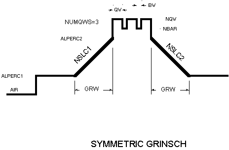
F. Symmetric Grinsch Structure
Modeig/II has a powerful symmetric Grinsch structure handling routine. To generate the layer information for a symmetric Grinsch structure use the parameter 'SYM=1'. The symmetric Grinsch routine requires the following parameters to be specified prior to the use of the 'SYM=1' flag: 'GRW', 'ALPERC1', 'ALPERC2', 'NSLC1', 'NSLC2', and 'NUMQWS'. This routine assumes that the graded width (GRW) is the same for both of the graded layers. The format for the symmetric Grinsch structure is:
STRUCT WVL=.7850 ! wavelength
STRUCT NQW=3.64 ! quantum well index (GaAs)
STRUCT QW=.0025 ! single quantum well width
STRUCT NBAR=3.42 ! barrier index
STRUCT BW=.0001 ! barrier width
STRUCT GRW=.1 ! graded width =.1 (microns)
STRUCT ALPERC1=.70 ALPERC2=.35 ! Al %
STRUCT NSLC1=10 NSLC2=10 ! # of slices
STRUCT NUMQWS=3 ! # of quantum wells
LAYER AIR=1.0 ! air layer effective index
LAYER SYM=1 ! symmetric Grinsch flag
(see App. 3 & Pict. 1)
Using the 'NUMQWS' parameter with the 'SYM=1' flag tells Modeig/II to generate the quantum well structure using the 'NQW', 'QW', 'NBAR', and 'BW' parameters. If a multiple quantum well structure is desired 'NBAR' and 'BW' must be defined before using the 'SYM=1' flag.
G. Asymmetric Grinsch Structure
Constructing an asymmetric Grinsch structure is almost identical to constructing a symmetric Grinsch structure. The only difference is Modeig/II will use two values for the graded widths ('GRW1' and 'GRW2'). These two values must be specified along with the other parameters mentioned in the symmetric Grinsch setup before the asymmetric Grinsch flag 'ASYM=1' is used. The format for the asymmetric Grinsch structure is:
STRUCT WVL=.7850 ! wavelength
STRUCT NQW=3.64 ! quantum well index (GaAs)
STRUCT QW=.0031 ! single quantum well width
STRUCT NBAR=3.42 ! barrier index
STRUCT BW=.0001 ! barrier width
STRUCT GRW=.1 GRW2=.2 ! graded widths
STRUCT ALPERC1=.70 ALPERC2=.35 ! Al %
STRUCT NSLC1=10 NSLC2=10 ! # of slices
STRUCT NUMQWS=3 ! # of quantum wells
LAYER AIR=1.0 ! air layer effective index
LAYER ASYM=1 ! asymmetric Grinsch flag
(see App. 3,4 & Pict. 2)
Using Appendix 4 as an example, all of the 'LAYER' input cards could be replaced by:
LAYER AIR=1.0 ! air layer effective index
LAYER ASYM=1 ! asymmetric Grinsch flag
Adding 'NUMQWS=3' to the 'STRUCT' input would create the same layer information as Appendix 4 in a much more concise format.
V. Near and Far Field Calculations
The near field and far field calculations are turned on by setting the 'NFPLT' and 'FFPLT' flags in the 'CASE' input card equal to one. The near field calculations must be made in order to calculate the far field, so if the far field calculations are selected the near field calculations will be made regardless of the current flag setting.
The full width half power calculations (FWHPN and FWHPF) will automatically be made according to the 'NFPLT' and 'FFPLT' flags. This data will be output to the '_dbase' file unless the 'FWHPNO' or 'FWHPFO' flags in the 'OUTPUT' card are set to zero.
The near field and far field data will be output to the files '_nfield' and '_ffield' respectively, if the calculations are made. These files can be suppressed by setting the 'NFOUT' or 'FFOUT' flags in the 'OUTPUT' card equal to zero. The '_nfield' and '_ffield' file data is in tab delimited columnar format with column headers and a leading asterisk, this format is the standard for use with some graphics software packages (i.e. Cricket Graph), or the files can be cut and pasted into a graphics package.
The near field and far field data can also be listed to the '_output' file by setting 'PRINTF' in the 'CASE' input card equal to one. The default is 'PRINTF' equal to zero, no listing of the field data in the '_output' file.
VI. Confinement Factor Calculations (Gamma)
The confinement factor (gamma) calculation is always turned on. The 'LAYGAM', 'GAMALL', and 'COMPGAM' flags in the 'GAMOUT' input card determine what calculations will be made. The 'LAYGAM' flag specifies for which layers of the structure gamma will be calculated and output to the '_dbase' file. The format for using the 'LAYGAM' flag is:
GAMOUT LAYGAM=1-4,6,8-10 ! layers 1,2,3,4,6,8,9,10
(see App. 1)
The '-' (dash) character is used as an inclusive separator while the ',' (comma) character is used as an and separator. In this example gamma will be calculated and output to the '_dbase' file for the layers 1,2,3,4,6,8,9,10.
While the 'LAYGAM' flag is used to tell Modeig/II which gammas to output to the '_dbase' file, the 'GAMALL' flag is used for the '_output' file. If 'GAMALL' is set equal to zero, the '_output' file will contain the gammas specified in the 'LAYGAM' flag. If 'GAMALL' is set equal to one the '_output' file contains the gammas for all the layers in the structure.
The 'COMPGAM' flag is used for the complex gammas. If 'COMPGAM' is set equal to zero, the complex gammas will not be calculated. If 'COMPGAM' is set equal to one the complex gammas for the layers specified by the 'GAMALL' and 'LAYGAM' flags will be calculated. The complex gammas appear only in the '_output' file.
The precision of the gamma calculations is controlled by the 'GAMEPS' parameter in the 'CASE' input card. The format for the 'GAMEPS' parameter is:
CASE GAMEPS=1E-3 ! gamma precision (3 digits)
In this example there will be 3 digits of accuracy (1E-3) in the gamma calculations.
VII. Looping
A. Low-level (X looping)
Modeig/II has the ability to do low-level (X) looping on the layer level. The 'ILX', 'FINV', 'XINC', and 'LAYCH' parameters in the 'LOOPXn' input card must be specified in order to do low-level looping. The 'ILX' parameter specifies which layer parameter ('TL', 'NREAL', 'NLOSS') to loop and must be first in the 'LOOPXn' input card. 'ILX' can be defined using either an integer or a character string to represent the loop variable. The following table can be used to define the 'ILX' parameter:
ILX = 0 or 'OFF' ! no looping
ILX = 1 or 'TL' ! loop on thickness (TL)
ILX = 2 or 'NREAL' ! loop on effective index (NREAL)
ILX = 3 or 'NLOSS' ! loop on the loss (NLOSS)
The 'FINV' parameter specifies the final value of the loop variable when the looping is completed. The 'XINC' parameter specifies the loop increment and must be negative if the loop variable is to be decremented. The 'LAYCH' parameter is used to specify the layer number of the variable to be looped. The following format should be used for low-level (X) looping:
LAYER2 TL=1.0
LOOPX1 ILX='TL' XINCR=-.1 FINV=0.00 LAYCH=2
In this example Modeig/II will loop on the thickness of the second layer of the structure, decrementing by .1 until the thickness equals 0.00 microns. The initial values for all low-level loop parameters are defined in the 'LAYER' input cards.
The number '1' appended to the 'LOOPX' input card is used to specify the order of looping. A maximum of 40 simultaneous and 40 nested loops are possible, allowing up to 1600 loops. To specify simultaneous loops use the same loop number:
LAYER2 NREAL=3.60 TL=1.0 ! simultaneous loops
LOOPX1 ILX='TL' XINCR=-.1 FINV=0.00 LAYCH=2
LOOPX1 ILX='NREAL' XINCR=.01 FINV=3.64 LAYCH=2
To specify nested loops use incremented loop numbers:
LAYER2 NREAL=3.60 TL=1.0 ! nested loops
LOOPX1 ILX='TL' XINCR=-.1 FINV=0.00 LAYCH=2
LOOPX2 ILX='NREAL' XINCR=.01 FINV=3.64 LAYCH=2
The loop procedure for nested looping follows this format:
LOOPX1
LOOPX2
LOOPX3
END LOOPX3
END LOOPX2
END LOOPX1
B. High-level (Z looping)
Modeig/II also has the ability to perform high-level (Z) looping which is looping on the structure level. The input parameters and format are very similar to those used for low-level (X) looping. The 'ILZ', 'FINV', and 'ZINC' parameters correspond to the 'ILX', 'FINV', and 'XINC' parameters of low-level looping. The 'ILZ' parameter specifies which structure parameter (see table below) to loop and must be first in the 'LOOPZn' input card. 'ILZ' can be defined using either an integer or a character string to represent the loop variable. The following table can be used to define the 'ILZ' parameter:
ILZ = 0 or 'OFF' ! no looping
ILZ = 1 or 'WVL' ! loop on wavelength (WVL)
ILZ = 2 or 'GRW' ! loop on graded width (GRW)
ILZ = 3 or 'QW' ! loop on quantum well width (QW)
ILZ = 4 or 'NQW' ! loop on quantum well index(NQW)
ILZ = 5 or 'ALPERC1' ! loop on aluminum percentage 1
ILZ = 6 or 'ALPERC2' ! loop on aluminum percentage 2
ILZ = 7 or 'ALPERC3' ! loop on aluminum percentage 3
ILZ = 8 or 'ALPERC4' ! loop on aluminum percentage 4
ILZ = 9 or 'GRW2' ! loop on graded width 2
ILZ = 10 or 'GRW3' ! loop on graded width 3
ILZ = 11 or 'GRW4' ! loop on graded width 4
ILZ = 12 or 'NSLC1' ! loop on number of slices 1
ILZ = 13 or 'NSLC2' ! loop on number of slices 2
ILZ = 14 or 'BW' ! loop on barrier width
ILZ = 15 or 'NBAR' ! loop on barrier index
ILZ = 16 or 'NUMQWS' ! loop on number of quantum wells
ILZ = 17 or 'QZMR' ! loop on initial guess (real part)
ILZ = 18 or 'QZMI' ! loop on initial guess (imag part)
The 'FINV' parameter specifies the final value of the loop variable when the looping is completed. The 'ZINC' parameter specifies the loop increment and must be negative if the loop variable is to be decremented. The following format should be used for high-level (Z) looping:
STRUCT WVL=.7850
LOOPZ1 ILZ='WVL' XINCR=.005 FINV=.8100
In this example Modeig/II will loop on the wavelength incrementing by .005 until the wavelength equals the final value .8100 angstroms. The initial values for all high-level loop parameters are defined in the 'STRUCT' input cards.
The number '1' appended to the 'LOOPZ' input card is used to specify the order of looping. A maximum of 20 simultaneous and 20 nested loops are possible, allowing up to 400 loops. To specify simultaneous loops use the same loop number:
STRUCT WVL=.7850 GRW=.1
LOOPZ1 ILZ='WVL' XINCR=.005 FINV=.8100
LOOPZ1 ILZ='GRW' XINCR=.05 FINV=.3
To specify nested loops use incremented loop numbers:
STRUCT WVL=.7850 GRW=.1
LOOPZ1 ILZ='WVL' XINCR=.005 FINV=.8100
LOOPZ2 ILZ='GRW' XINCR=.05 FINV=.3
The loop procedure for nested looping follows this format:
LOOPZ1
LOOPZ2
LOOPZ3
LOOPX1
LOOPX2
LOOPX3
END LOOPX3
END LOOPX2
END LOOPX1
END LOOPZ3
END LOOPZ2
END LOOPZ1
C. Initial Guess Generation
Modeig/II has the ability to generate initial guesses (QZMR, QZMI) to find the fundamental mode (PHM<1) in the root search.
The initial guess generation routine only works for structures with single quantum wells, the index and thickness of the layer directly preceding the quantum well is used for the calculation.
The 'INITGS' flag in the 'CASE' input card must be set to one to invoke this routine, otherwise the initial guess must be directly input using the 'QZMR' and 'QZMI' parameters in the 'CASE' input card. 'QZMR' is the real part of the initial guess and 'QZMI' is the imaginary part. The format for automatic initial guess generation is:
CASE INITGS=1 ! initial guess generation
(see App. 2,3)
The format for direct input of the initial guess is:
CASE INITGS=0 ! turn off initial guess generation
CASE QZMR=10.9 QZMI=0.00 ! direct input guess
(see App. 1,4)
D. Wavelength vs. Quantum Well Width
When looping on the wavelength (WVL) it may be necessary to update the quantum well width with each increment of the wavelength. There are two ways of doing this, one is to use the automatic quantum well generation routine described in a previous chapter or to loop on the quantum well width simultaneously. Looping on the quantum well width will automatically turn off the quantum well width generation routine.
(see Auto Quantum Well Width Calculation, IV. E)
E. Multiple Output File Generation
When doing any looping it is possible to store the output into multiple sets of files instead of just the one set of output files ('_dbase', '_output', ...). Setting the 'SPLTFL' flag in the 'OUTPUT' card greater than zero will cause Modeig/II to split the output into multiple files with the looping variables appended onto the filenames. See the General Information section in the Output section of this manual.
VIII. Output
A. Output File General Information
There are 5 possible output file types created by Modeig/II:
_dbase - Output parameters plot file
_layers - Input file layer information
_output - running account of program operation
_nfield - near field plot file
_ffield - far field plot file
The filenames for these file types are created by taking the input file filename, or the entered output filename (see General Operation), and appending the file type suffix to the end. For example:
input filename: inputfile
output filenames: inputfile_dbase
inputfile_layers
inputfile_output
inputfile_nfield
inputfile_ffield
If looping is being performed a multiple file option is available. Setting the 'SPLTFL' flag in the 'OUTPUT' card greater than zero will cause Modeig/II to store the data in multiple output files. Modeig/II will use the looping variables as suffixes to the output filenames, every pass through a loop will create a new output file. The 'SPLTFL' flag can have the following values:
SPLTFL=0 ! single output file
SPLTFL=1 ! multiple output files with lowest order loop intact
SPLTFL=2 ! multiple output files for every loop variable
An example is:
inputfile:
STRUCT WVL=.7900
OUTPUT MODOUT=0 NFOUT=0 FFOUT=0
OUTPUT SPLTFL=1
LOOPZ1 ILZ='WVL' FINV=.7950 ZINCR=.005
input filename: inputfile
output filenames: inputfile_dbase_7900
inputfile_layers_7900
inputfile_dbase_7950
inputfile_layers_7950
The '_nfield' and '_ffield' output files are created only if the near and far field calculation flags are set equal to one (NFPLT and FFPLT, respectively). The '_dbase', '_layers', and '_output' files are created automatically by Modeig/II and will be created for every case unless their output flags are set to zero. To deselect any of the 5 output files or the screen output set its corresponding output flag to zero. The output files and their corresponding output flags are:
_dbase - DBOUT
_layers - LYROUT
_output - MODOUT
_nfield - NFOUT
_ffield - FFOUT
screen - SCROUT
B. Dbase File
The '_dbase' file is the output file which contains the looping variables and these 8 output parameters:
1) PHM - Phase integral
2) GAMMA - Confinement factor
3) WZR - Eigenvalue root (real part)
4) WZI - Eigenvalue root (imaginary part)
5) QZR - WZR squared
6) QZI - WZI squared
7) FWHPN - Near field full width half power
8) FWHPF - Far field full width half power
The '_dbase' file will be created automatically by Modeig/II. If the '_dbase' file is not needed it can be turned off by setting the 'DBOUT' flag in the 'OUTPUT' card equal to zero.
The '_dbase' output file is in tab delimited columnar format with column headers and a leading asterisk. This format is used for input files by many graphics software packages (i.e. Cricket Graph) so graphical outputs are easily obtained.
The '_dbase' file can be customized by selecting or deselecting output parameters using their corresponding output flags. The output flags are in the 'OUTPUT' card and are formed by appending the character 'o' to the end of the parameter name. An example is:
OUTPUT PHMO=0 WZRO=1
In the above example the output parameter PHM is deselected and will not be output to the '_dbase' file, the parameter is still calculated and can be output to another file. The output parameter WZR is selected and will be output to the '_dbase' file. The 8 possible output flags are:
1) PHMO ! ( 0= deselect, 1= select)
2) GAMMAO
3) WZRO
4) WZIO
5) QZRO
6) QZIO
7) FWHPNO
8) FWHPFO
The column order for the '_dbase' output is pre-defined. The high-level looping variables (WVL,GRW,...) are listed first in the order in which the looping takes place. The low-level looping variables (TL,NREAL,NLOSS) are listed next and are also output in the order in which the looping takes place. Finally, the 8 output parameters are listed depending upon their output flags. The order of precedence of the 8 output flags is the order in which they are listed in the above tables.
The low-level looping variables and the output parameter GAMMA can have output for more than one layer. The column headers for these outputs will contain the parameter name with the layer number, in parentheses, appended to the end. An example is:
TL(1) TL(2) GAMMA(1) GAMMA(2) PHM
If using the multiple files option (SPLTFL=1), Modeig/II will use the high-level looping variables as suffixes to the output filename. To avoid redundancy and compress the '_dbase' file, the high-level looping variables will not be listed in the '_dbase' file when this option is selected, since the looping variables appear in the filenames.
An example of the '_dbase' file is 'Appendix1_dbase' located at the back of this manual.
C. Layers File
The '_layers' file contains the effective index, loss, and layer thickness for each layer generated from the 'STRUCT' and "layer' input cards in the input file. A new set of layer information is generated each time Modeig/II goes through a high-level loop, so for each loop the loop variables and the layer information are output to the '_layers' file. If the multiple files option is selected (SPLTFL=1), Modeig/II will create a new '_layers' file each time it passes through a high-level loop, appending the loop variable to the filename as described in the '_dbase' file chapter.
This file is intended to be used as a check to see if Modeig/II is generating the proper layer information and as an record of the cases run. If the '_layer' file is not desired it can be turned off by setting the 'LYROUT' flag in the 'OUTPUT' card to zero.
An example of the '_layers' file is 'Appendix1_layers' located at the back of this manual.
D. Output File
The '_output' file is a running account of the input, calculations, and output that is being used by Modeig/II. the '_output' file can contain an enormous amount of information, if the '_output' file is not desired it can be turned off by setting the 'MODOUT' flag in the 'OUTPUT' card to zero. The data that will be stored in the '_output' file can be controlled using a number of parameters in the 'CASE' input card, for further information see the Variable Glossary at the back of this manual.
An example of the '_output' file is 'Appendix1_output' located at the back of this manual.
E. Nfield File
The '_nfield' file is the output file which contains the near field data. The 5 near field output parameters are:
XXFT - X location
NFINT - Near field intensity
PHASE - Near field phase
NFREAL - Near field (real part)
NFIMAG - Near field (imag part)
The '_nfield' file will be automatically created when the near field or far field calculation flags are set to one (NFPLT or FFPLT).
The '_nfield' output file is in tab delimited columnar format with column headers and a leading asterisk. This format is used for input files by many graphics software packages (i.e. Cricket Graph) so graphical outputs are easily obtained.
An example of the '_nfield' file is 'Appendix1_nfield' located at the back of this manual.
F. Ffield File
The '_ffield' file is the output file which contains the far field data. The 5 far field output parameters are:
THETA - X location
FFIELD - Far field
PHASE - Far field phase
The '_ffield' file will be automatically created when the far field calculation flag is set to one (FFPLT).
The '_ffield' output file is in tab delimited columnar format with column headers and a leading asterisk. This format is used for input files by many graphics software packages (i.e. Cricket Graph) so graphical outputs are easily obtained.
An example of the '_ffield' file is 'Appendix1_ffield' located at the back of this manual.
Variable Glossary
CASE PARAMETERS
ALPHAA - Coefficient used in the computation of G(Y) and Neff (0.019)
AUTOQW - Automatic quantum well width calculation flag (0)
BL - Amount of offset for the left side of the region of applied current (4)
BM - Amount of offset for the center of the region of applied current (0)
BR - Amount of offset for the right side of the region of applied current (-1D-10)
DELTA - Delta used in the computation of the current (0.5)
DELTAL - value of delta for the left side (0.5)
DELTAR - value of delta for the right side (-1D-10)
DTHETA - Increment for the far field angle theta (1.0)
DXIN - Dx used for fine detail in near field (0.1)
EPS1 - Epsilon for convergence test on delta QZ root search (1E-8)
EPS2 - Epsilon for convergence test on magnitude of eigen equation function (1E-8)
FFPLT - Far field calculation flag (0)
GAMEPS - Confinement factor (Gamma) accuracy epsilon (1E-3)
GCOEFF - Coefficient used to compute gain from current density (0.0045)
IDEN - Density of points in X for field calculations per rad or 1/E (10)
IL - Iteration limit maximum number for each root search (30)
IMAX - maximum number of points in each layer for field calculations (not applicable if DXIN is used) (15)
INFX - number of rad or 1/e dist into semi-infinite layers for field calculations (3)
INITGS - Initial guess generation routine flag (0)
INTHM - Half maximum intensity level (0)
JE - Peak current density (within window) (0.0)
KASE - Modeig/II case number (yy/mm/dd)
KCI - Complex freq factor for normalized KO (imag part) (0.0)
KCR - Complex freq factor for normalized KO (real part) (1.0)
KDOF - Subroutine Fields flag: (1)
0 = No field calculations made
1 = Tangential fields at boundaries only calculated
2 = Fields as a function of X calculated iff KOUT=4
KDOFY - Option for computing fields as function of y (1)
(similar to usage of KDOF for x-modes)
note ... if the near field or the far field is to be
calculated (and perhaps plotted) as a function of y
for 2-d problems (i.e. when LXYOPT = 1),
then KDOFY must be 2 and KOUFY must be 3 or 4.
KEIF - control type of eigen equation used for root searching:
1 = unmodified eigen equation from SM matrix
2 = eigeqf renormalized to R.M.S. Mag. of the 4 possible eigeqf
3 = Eigeqf multiplied by WT function to bias search toward intended MM. Weight function is WFMP times squared difference between phase integral index and intended mode index.
Warning: 2&3 are non-analytic functions, can greatly slow root search
KFI - Explicit complex freq factor (imag part)
KFR - Explicit complex freq factor (real part)
KGCZ - Control use of guesses in cmplx root search for all QZ. used to set KM= KGCZ for all guesses. (KGSS.ge.2)
=0 guesses not used, initial iterates about point (1.0,0.0)
=1,2,3 initial iterates at radius of 0.1**KGCZ about each guess.
only converged and iteration limited roots divided out.
=4,5,6,7 radius of 0.1**KGCZ, all other guesses and roots divided out
Warning: Use KGCZ.ge.4 iff guesses are good approx and distinct.
do not use if all guesses the same (KGSS=2) or poor input guess.
if good guesses, KGCZ.ge.4 greatly speeds root search convergence.
KGCZY - Option to control use of estimates for y-modes (3)
(similar in use to KGCZ)
KGSS - Control type of initial guesses for QZ root search. (3)
=1 QZM(M) and KM(M) from input or previous case used for guesses,
=2 all guesses the same (QR max of inner layers),
=3 individual guesses from simple quadratic approx for real(QZ) vs phase integral. intended mode indices MM= MO+M.
KGSSY - Option for obtaining estimates for y-roots (see KGSS)
KM(M) - Index showing QZM quality or type. (5)
input value used only if KGSS=1.
=0 to 7, see KGCZ
=8 QZM used as fixed known root, no search, divided out for others
(for output and prev case KM= 5,6,7, shows type of convergence)
KMDO - Modes are output and fields calculated only for KM.ge.KMDO (5)
KO - Free-space propg const for normalization purposes.
(calculated quantity rather than input)
KO= 2PI/WVL used to norm all propg consts. see KC below.
effective values of WVL and KO altered by use of non-unity KC.
KOUE - Flag to control output from subroutine Eigeqf 1-4 (0)
KOUF - Flag to control output from subroutine Fields 1-4 (3)
KOUFY - Option for outputting fields as function of y (3)
KOUI - Flag to control output from subroutine Putsin 1-4 (1)
KOUS - Flag to control output from subroutine Search 1-4 (3)
KOUZ - Flag to control output from subroutine Czerom 1-4 (3)
KXTL - Control to specify that XL or TL are expected as input (0)
.le. 0 if XL expected as input, TL calculated. (default)
.ge. 1 if TL expected as input, XL calculated. XL(1)= 0.
LAYER - Finite layer over which numer. integral is performed (2)
in fldint (active layer)
modified 9/85
numerator integral is now performed for all finite layers.
layer now just represents the active layer used in cxmode.
LCL - Left spreading factor for the center section (6.)
LCR - Right spreading factor for the center section (6.)
LCUTOF(M)- Field cutoff criterion for left margin for mode M (-1.D10)
fy(x) = 0 for x .lt. LCUTOF(M) or for x .gt. XCUTOF(M)
LLEFT - Current spreading parameter for the left portion (0.025)
LRIGHT - Current spreading parameter for the right portion(0.025)
LXYOPT - Effective index of refraction option (0)
= 1 if effective index of refraction option is desired
to solve 2-dimensional problem.
= 0 otherwise. (normal 1-d problem)
MN - Number of x-modes to be searched for or calculations made (1)
maximum number of modes presently dimensioned for is 10.
for 2-d problem (LXYOPT = 1) the maximum value of MN is 3.
MNY - Number of modes desired for y-direction (2)
MNY must be .le. 10)
MO - Bias for mode indexing of intended modes. MM=MO+M (-1)
NBARFF - N bar used in the far field calculations (3.45)
NFPLT - = 1 to plot near field, = 0 otherwise. (0)
NY - Number of y-slices (no default value, must be specified)
PEROPT - Option for specifying PER(l) and PEI(l): (0)
if = 0, then PER(l) and PEI(l) are input directly
if = 1, then PER(l) and PEI(l) are computed from the input quantities NREAL(l), NLOSS(l), and GAIN0.
PFIELD - Field power used to normalize the field fy(x) (1.)
PMFR - Fract. part for phase integral (phase shift at outer bdy)
assumed in generating guesses. units of pi. (0.3)
PMI(1) - Relative permeability, imag part, all layers (0.0)
PMR(1) - Relative permeability, real part, all layers (1.0)
PRINTF - Control for printing table of fields,intensities,
and phases (0)
QCNT - Mode index used for the input of multiple mode initial
guesses (QZMR(QCNT)= ...) (1)
QZMR - Input set of complex QZ values (x-modes) M= 1,MN QZMI see KGSS=1.
used for guesses for root search, or for field calc, no search. preset to special real values from default case solutions.
if LXYOPT = 0, then MN .le. 10 values may be specified.
if LXYOPT = 1, then MN .le. 3 values may be specified.
(use QCNT for multiple input)
QZNI - Imag part of QZ for generation of initial guesses (-1.D-4)
QZNR - Real part of QZ for generation of initial guesses (0.9)
RAT - Rat factor, used in the computation of n eff (-2.)
ALPHAA coefficient used in the computation of g(y) and n eff (0.019) (also called ALPHAA)
SPREAD - Current spreading parameter (l0) (same as LCL) (6.)
WC - Current window width (2E-10)
WFMP - WT funct multiplier used for modified eigen eq funct. (100.0)
WL - The width of the left portion of the region (5.5)
WR - The width of the right portion of the region (5.5)
XAXLEN - X-axis length (inches) (10.0)
XCUTOF(M) - Field cutoff criterion for right margin for mode M (1.D10)
XU - Unit of length implied for all dimensions (meters) (1E-6)
YAXLEN - Y-axis length (inches) (5.0)
YESTR - Estimates for eigenvalues (modes) in y-direction
YESTI (complex)
(no default estimates are provided. estimates must
be provided if LXYOPT = 1)
MODCON PARAMETERS
APB1 - Principal branch specification for wx-planes. Angle
APB2 into WX half plane for outer layers L1 and L2+1. units of pi. (0.25)
(direction angle of branch cuts in QZ plane is twice APB.)
+0.0.le.APB.le.+1.0 branch includes pos imag axis of wx- plane.
-0.5.le.APB.le.+0.5 branch includes pos real axis of wx- plane.
default APB1=0.25, APB2=0.25, not conventional specification.
rather, imag(wx).ge.real(wx). bound and leaky mode roots for lossless dielectic structures are all on same principal branch. Branch cuts in QZ plane are in pos imag direction. (conventional choice of branches, APB=0.5, KBD=2. bound proper mode roots on principal branch and Riemann sheet of QZ. leaky improper mode roots on second branch and riemann sheet. Branch cuts in QZ plane in negative real direction.)
F1 - Determines how far the integration range will extend into layer 1 or layer LN, respectively (see subroutine fldint)
KBC1 - Control type of boundary conditions at 1-st and last bdy L1,L2.KBC2 open-bdy semi-inf wave admit/imped, or fixed surf admit/imped, also eigen, non-eigen, conditions, and acceptable solutions.
le.0 open boundary condition, non-eigen condition, no search made.
inward and outward soln both acceptable seeKBD1,KBD2
field soln exits for each of KBC1=0, or KBC2=0, or both.
if both, two indeped field soln exist. calc independ from two bdy cond same as for KBC=1, and direction implied by KBD1,KBD2.
=1 open boundary, eigen condition. only a single exponential wave solution acceptable in outer semi-inf layer. (default)
=0,1 wave admit/imped for semi-inf layer is funct of wx(qz), always defined from wx on principal branch. see KBD1,2 and APB1,2
=2 closed bdy, a fixed surf admit/imped YB1,YB2. ZB1,ZB2 ignored
=3 closed bdy, a fixed surf imped/admit ZB1,ZB2. YB1,YB2 ignored
=2,3 a closed bdy eigen cond. outer semi-inf layers ignored.
KBD1 - Controls implied direction of single soln in semi-inf KBD2 layers inward/outward direction interpretation depends on branch def.
KBD1=1 pos. exponent (inward) complex wave solution in layer L1
KBD1=2 neg. exponent (outward) complex wave solution in layer L1
KBD2=1 neg. exponent (inward) complex wave solution in layer L2+1
KBD2=2 pos. exponent (outward) complex wave solution in layer L2+1
default values KBD1=2,KBD2=2. outward soln in semi-inf layers.
iff APB= 0.5, then imag(wx) is pos, and direction sense in/out is that of exp decay regardless of phase propag. inward= leaky, improper or incomming lossy wave. outward= bound, proper or out going lossy wave. iff APB= 0.0, real(wx) is pos. and direction is that of phase propagation regardless of exp decay or growth. direction sense also used for non-eigen case (KBC1,KBC2=0) in generating solutions based on each bdy cond independently. KBD. also used for direction sense for YB,ZB surf admit/imped.
KPOL - Polarization. transv to z-propg, and to x-norm direct. (1)
.le.1 te, transverse electric case. fy= ey. (default)
.ge.2 tm, transverse magnetic case. fy= hy
L1 - First and last boundary for outer boundary conditions.
L2 preset to L1=1, L2=LN-1 for each case.
for other values (partial structures), L1,L2 must be input
for each successive case.
note. adjacent layers (l= L1 and L2+1) are taken to be
semi-infinite for closed bdy cond. (KBC=2,3). all outer layers ignored.
YB1R, YB1I - Fixed bdy surface admit(te)/imped(tm) looking
YB2R, YB2I outward at L1,L2. Used only if respective KBC1,KBC2 are equal to 2 (1.0,0.0)
ZB1R, ZB1I - Fixed bdy surface imped(te)/admit(tm) looking outward ZB2R, ZB2I at L1,L2. Used only respective if KBC1,KBC2 are equal to 3. (1.0,0.0)
looking outward iff KBD1,2 equal 2 (default)
STRUCT PARAMETERS
ALPERC1 - First aluminum percentage
ALPERC2 - Second aluminum percentage
ALPERC3 - Third aluminum percentage
ALPERC4 - Fourth aluminum percentage
BALPERC - Barrier aluminum percentage
BW - Barrier width
GRW - Graded layer width
GRW1 - Width of the first graded layer
GRW2 - Width of the second graded layer
GRW3 - Width of the third graded layer
GRW4 - Width of the fourth graded layer
LGRAD - layer number at the start of the graded layer
LN - total number of layers in the structure
LSTART - starting layer number for the structure
NBAR - Barrier effective index
NQW - Quantum well effective index
NSLC1 - Number of slices for first graded layer
NSLC2 - Number of slices for second graded layer
NUMQWS - Number of quantum wells
QW - Quantum well width
QWALPERC - Quantum well aluminum percentage
LAYER PARAMETERS
AIR - Air layer effective index
ALPERC - Aluminum percentage
ASYM - Asymmetric Grinsch structure flag
BALPERC - Barrier aluminum percentage
BARRIER - Barrier effective index
BW - Barrier width
GRW - Graded layer width
NLOSS - Loss
NREAL - Effective index
NSLC - Number of slices for the graded layer
NUMQWS - Number of quantum wells
QW - Quantum well width
QWALPERC - Quantum well aluminum percentage
SYM - Symmetric Grinsch structure flag
GAMOUT PARAMETERS
COMPGAM - Complex confinement factor (gamma) flag
GAMALL - Gamma layers to output to output file
LAYGAM - Gamma layers to output to dbase file
LOOPX PARAMETERS
FINV - Final value of the of the loop variable when looping
ILX - Loop variable selection flag
0 or 'OFF' = no looping
1 or 'TL' = loop on thickness (TL)
2 or 'NREAL' = loop on effective index (NREAL)
3 or 'NLOSS' = loop on the loss (NLOSS)
LAYCH - Layer number to loop on
XINC - Loop increment value
LOOPZ PARAMETERS
FINV - Final value of the of the loop variable when looping
ILZ - Loop variable selection flag
0 or 'OFF' = no looping
1 or 'WVL' = loop on wavelength (WVL)
2 or 'GRW' =loop on graded width (GRW)
3 or 'QW' = loop on quantum well width (QW)
4 or 'NQW' =loop on quantum well index(NQW)
5 or 'ALPERC1' = loop on aluminum percentage 1
6 or 'ALPERC2' = loop on aluminum percentage 2
7 or 'ALPERC3' = loop on aluminum percentage 3
8 or 'ALPERC4' = loop on aluminum percentage 4
9 or 'GRW2' = loop on graded width 2
10 or 'GRW3' = loop on graded width 3
11 or 'GRW4' = loop on graded width 4
12 or 'NSLC1' = loop on number of slices 1
13 or 'NSLC2' = loop on number of slices 2
14 or 'BW' = loop on barrier width
15 or 'NBAR' = loop on barrier index
16 or 'NUMQWS' = loop on number of quantum wells
17 or 'QZMR' = loop on initial guess (real part)
18 or 'QZMI' = loop on initial guess (imag part)
ZINC - Loop increment value
OUTPUT PARAMETERS
DBOUT - Dbase file output flag (1-enabled)
DPRINT - Dbase file auto print flag (0-disabled)
FFOUT - Far field file output flag (1-enabled)
FPRINT - Far field file auto print flag (0-disabled)
FWHPNO - Near field full width half power dbase output flag
FWHPFO - Far field full width half power dbase output flag
GAMMAO - Confinement factor (GAMMA) dbase output flag
LPRINT - Layer file auto print flag (0-disabled)
LYROUT - Layer file output flag (1-enabled)
MODOUT - Output file output flag (1-enabled)
NFOUT - Near field file output flag (0-disabled)
NPRINT - Near field file auto print flag (0-disabled)
OPRINT - Output file auto print flag (0-disabled)
PHMO - PHM (phase integral) dbase output flag (1-enabled)
QZIO - QZ root search (imag part) dbase output flag
QZRO - QZ root search (real part) dbase output flag
QZMIO - Initial guess (imag part) dbase output flag
QZMRO - Initial guess (real part) dbase output flag
SCROUT - Screen output flag (1-enabled)
SPLTFL - Multiple files flag (suffixes) (0-disabled)
WZIO - WZ (imag part) dbase output flag
WZRO - WZ (real part) dbase output flag
Appendices
Appendix 1
CASE KASE=890316
CASE QZMR=11.70014 QZMI=.003 EPS1=1E-7 GAMEPS=1E-3
CASE PRINTF=0 INITGS=0 AUTOQW=0 NFPLT=1 FFPLT=1
MODCON KPOL=1 APB1=0.25 APB2=0.25
STRUCT WVL=.8300
LAYER01 NLOSS= .00000 NREAL= 3.40000
LAYER02 NLOSS= .00000 NREAL= 3.62000 TL= 0.06000
LAYER03 NLOSS= .00000 NREAL= 3.40000 TL= .25000
LAYER04 NLOSS= .00000 NREAL= 3.40000 TL= .05000
LAYER05 NLOSS= .50000 NREAL= 3.64000 TL= .05000
LAYER06 NLOSS= .50000 NREAL= 3.64000
OUTPUT PHMO=1 GAMMAO=1 WZRO=1 WZIO=0 QZRO=1 QZIO=0
OUTPUT SPLTFL=0
GAMOUT LAYGAM=1 COMPGAM=0 GAMALL=0
1) Direct layer input (explicit)
2) Near/Far field calculations
Appendix 2
CASE KASE=890316
CASE EPS1=1E-7 GAMEPS=1E-3
CASE PRINTF=0 INITGS=1 AUTOQW=1 NFPLT=0 FFPLT=0
MODCON KPOL=1 APB1=0.25 APB2=0.25
STRUCT QW=.0031 NQW=3.64 GRW=.1 WVL=.7850
LAYER AIR=1.0
LAYER ALPERC=.70
LAYER ALPERC=.70
LAYER NSLC=10
LAYER ALPERC=.35
LAYER QWS=1
LAYER ALPERC=.35
LAYER NSLC=10
LAYER ALPERC=.70
LAYER ALPERC=.70 TL=0.0
OUTPUT PHMO=1 GAMMAO=1 WZRO=1 WZIO=0 QZRO=1 QZIO=0
OUTPUT FWHPNO=0 FWHPFO=0
OUTPUT SPLTFL=0 MODOUT=0
GAMOUT LAYGAM=14 COMPGAM=0 GAMALL=0
LOOPX1 ILX=1 FINV=0.90 XINC=-0.1 LAYCH=2
LOOPZ1 ILZ=1 FINV=.8100 ZINC=.005
LOOPZ2 ILZ=2 FINV=.3 ZINC=.1
1) Direct layer input (implicit)
2) Graded Layers
3) Auto Quantum Well Width calculation
4) Low-level (X) looping
5) High-level (Z) looping
6) Initial Guess generation
Appendix 3
CASE KASE=890316
CASE EPS1=1E-7 GAMEPS=1E-3
CASE PRINTF=0 INITGS=1 AUTOQW=1 NFPLT=0 FFPLT=0
MODCON KPOL=1 APB1=0.25 APB2=0.25
STRUCT NQW=3.64 NUMQWS=3 WVL=.7850
STRUCT NBAR=3.42 BW=.0001
STRUCT GRW=.1
STRUCT NSLC1=10 NSLC2=10
STRUCT ALPERC1=.70 ALPERC2=.35
LAYER AIR=1.0
LAYER SYM=1
OUTPUT PHMO=1 GAMMAO=1 WZRO=1 WZIO=0 QZRO=1 QZIO=0
OUTPUT FWHPNO=0 FWHPFO=0
OUTPUT SPLTFL=1 MODOUT=0
GAMOUT LAYGAM=14 COMPGAM=0 GAMALL=0
LOOPX1 ILX='TL' FINV=0.90 XINC=-0.1 LAYCH=2
LOOPZ1 ILZ='WVL' FINV=.7900 ZINC=.005
LOOPZ2 ILZ='GRW' FINV=.2 ZINC=.1
1) Direct layer input (implicit)
2) Graded Layers
3) Multiple Quantum Wells
4) Auto Quantum Well Width generation
5) Symmetric Grinsch Structure
6) Low-level (X) looping
7) High-level (Z) looping
8) Initial Guess generation
9) Multiple Files (suffixes)
Appendix 4
CASE KASE=890316
CASE QZMR=10.9 QZMI=.000 EPS1=1E-7 GAMEPS=1E-3
CASE PRINTF=0 INITGS=0 AUTOQW=0 NFPLT=0 FFPLT=0
STRUCT WVL=.7850
STRUCT QWALPERC=.16 QW=.0031
STRUCT BALPERC=.385 BW=.0001
STRUCT GRW1=.1 GRW2=.2
STRUCT NSLC1=10 NSLC2=10
STRUCT ALPERC1=.70 ALPERC2=.35
LAYER AIR=1.0
LAYER ALPERC=^1
LAYER ALPERC=^1
LAYER GRW=^1 NSLC=^1
LAYER ALPERC=^2
LAYER QW=.0031 QWALPERC=.16 ! quantum well (direct input)
LAYER BW=.0001 BALPERC=.385 ! barrier
LAYER QWS=2 ! two quantum wells (indirect input)
LAYER ALPERC=^2
LAYER GRW=^2 NSLC=^2
LAYER ALPERC=^1
LAYER ALPERC=^1 TL=0.0
MODCON KPOL=1 APB1=0.25 APB2=0.25
OUTPUT PHMO=1 GAMMAO=1 WZRO=1 WZIO=0 QZRO=1 QZIO=0
OUTPUT SPLTFL=0 MODOUT=0
GAMOUT LAYGAM=14 COMPGAM=0 GAMALL=0
LOOPX1 ILX='TL' FINV=0.90 XINC=-0.1 LAYCH=2
LOOPZ1 ILZ='WVL' FINV=.7900 ZINC=.005
LOOPZ1 ILZ='QW' FINV=.0040 ZINC=.0001
1) Direct Layer input (implicit)
2) Indirect Layer input (pointers)
3) Graded Layers
4) Multiple Quantum Wells
5) Asymmetric Grinsch Structure
6) Low-level (X) looping
7) High-level (Z) looping
Appendix1_dbase
PHM GAMMA( 1) WZR QZR FWHPN FWHPF
3.746032E-01 5.628879E-01 3.409635E+00 1.162559E+01 3.098492E-01 3.530000E+01
Appendix1_layers
# of layers = 6
LAYER01 NLOSS= .00000 NREAL= 3.40000 TL= .00000
LAYER02 NLOSS= .00000 NREAL= 3.62000 TL= .06000
LAYER03 NLOSS= .00000 NREAL= 3.40000 TL= .25000
LAYER04 NLOSS= .00000 NREAL= 3.40000 TL= .05000
LAYER05 NLOSS= .50000 NREAL= 3.64000 TL= .05000
LAYER06 NLOSS= .50000 NREAL= 3.64000 TL= .00000
******************************************************
Appendix1_output
1*************************************** PROGRAM MODEIG ****************************************
* * * * * * * * CALCULATION OF GENERAL COMPLEX*16 EIGEN-WAVES IN LAYERED STRUCTURES * * * * * * * *
CASE NO. 890316. 1
SUMMARY OF LAYERED STRUCTURE, POLARIZATION, ANDBOUNDARY CONDITIONS./
IMPLIED UNIT OF LENGTH XU= 0.10000D-05 METERS (BUT NOT USED EXPLICITLY). ALL QUANTITIES NORMALIZED.
NOMINAL WAVELENGTH WVL= .83000 XU, AND FREE-SPACE KO= 2PI/WVL= 7.57010 RAD/XU.
COMPLEX FREQUENCY FACTOR KC= ( 1.00000, .00000). EFFECTIVE-KO= KC*KO= ( 7.57010, .00000).
ALL PROPAGATION COEFFICIENTS ARE NORMALIZED TO EFFECTIVE-KO. (WAVE AND MATERIAL REFRACTIVE INDICES, IF KF= UNITY)
(WAVE ADMITTANCE(TE) AND IMPEDANCE(TM), YX AND YZ, ARE NORMALIZED TO THAT OF FREE SPACE.
NORMALIZED FREQUENCY KF= ( 1.00000, .00000)= FREQ/C*EFF.KO.
POLARIZATION, KPOL= 1 ( =1 TE CASE, =2 TM CASE)
TRANSVERSE ELECTRIC CASE. EX=HY=EZ=0. TANGENTIAL FY=+EY, FZ=+HZ. TRANSVERSE FX=-HX, FY=+EY. LONGITUDINAL FZ=+HZ.
YX=FZ/FY=+HZ/EY, AND YZ=FX/FY=-HX/EY, ARE WAVE ADMITTANCES. (IN THE POS X, Z, OR WAVE DIRECTION).
LAYERED STRUCTURE. 6 LAYERS TOTAL. 5 BOUNDARIES. 4 FINITE LAYERS.
PE=( 11.56000, .00000) PM=( 1.00000, .00000)
L 1 SEMI-INFINITE QN=( 11.56000, .00000) YN=( 1.00000, .00000)
RN=( 3.40000, .00000)
L1= 1---BOUNDARY FOR FIRST BOUNDARY CONDITION------------------------------------------
--L 1---XL= .00000---------------------------------------------------------
PE=( 13.10440, .00000) PM=( 1.00000, .00000)
L 2 TL= .06000 QN=( 13.10440, .00000) YN=( 1.00000, .00000)
( .07229WVL) RN=( 3.62000, .00000) PH0=( 1.64423, .00000)
--L 2---XL= .06000---------------------------------------------------------
PE=( 11.56000, .00000) PM=( 1.00000, .00000)
L 3 TL= .25000 QN=( 11.56000, .00000) YN=( 1.00000, .00000)
( .30120WVL) RN=( 3.40000, .00000) PH0=( 6.43459, .00000)
--L 3---XL= .31000---------------------------------------------------------
PE=( 11.56000, .00000) PM=( 1.00000, .00000)
L 4 TL= .05000 QN=( 11.56000, .00000) YN=( 1.00000, .00000)
( .06024WVL) RN=( 3.40000, .00000) PH0=( 1.28692, .00000)
--L 4---XL= .36000---------------------------------------------------------
PE=( 13.24524, .48084) PM=( 1.00000, .00000)
L 5 TL= .05000 QN=( 13.24524, .48084) YN=( 1.00000, .00000)
( .06024WVL) RN=( 3.64000, .06605) PH0=( 1.37776, .02500)
--L 5---XL= .41000---------------------------------------------------------
L2= 5---BOUNDARY FOR SECOND BOUNDARY CONDITION------------------------------------------
PE=( 13.24524, .48084) PM=( 1.00000, .00000)
L 6 SEMI-INFINITE QN=( 13.24524, .48084) YN=( 1.00000, .00000)
RN=( 3.64000, .06605)
FIRST BOUNDARY CONDITION. L1= 1, KBC1= 1, KBD1= 2.
OPEN BOUNDARY, SEMI-INFINITE ADJACENT LAYER.
PRINCIPAL BRANCH SPECIFICATION FOR WX. ANGLE APB= .250 PI, VECTOR VPB=( .707, .707), (WX*DOT*VPB.GE.0).
EIGEN CONDITION. OUTWARD WAVE SOLUTION ONLY. (DIRECTION OF DECAY IF IM(WX).GT.0, OF PHASE PROPAGATION IF RE(WX).GT.0.)
SECOND BOUNDARY CONDITION. L2= 5, KBC1= 1, KBD2= 2.
OPEN BOUNDARY, SEMI-INFINITE ADJACENT LAYER.
PRINCIPAL BRANCH SPECIFICATION FOR WX. ANGLE APB= .250 PI, VECTOR VPB=( .707, .707), (WX*DOT*VPB.GE.0).
EIGEN CONDITION. OUTWARD WAVE SOLUTION ONLY. (DIRECTION OF DECAY IF IM(WX).GT.0, OF PHASE PROPAGATION IF RE(WX).GT.0.)
END STRUCTURE DESCRIPTION.
****SUBROUTINE SEARCH. KASE NO.=890316. 1, KDOS= 1, KOUS= 3.
SEARCHING FOR MN= 1 EIGENVALUES. FOR INTENDED MODE INDICES FROM MM=MK= 0 TO MM=ML= 0.
REPRESENTATIVE VALUES OF REAL QZ AND CORRESPONDING PHASE INTEGRAL
QZR= .00000, .90000, 8.70871, 13.24524,
PHM= 3.41976PI, 3.28870PI, 1.78075PI, .05908PI,
KGSS= 1. INITIAL GUESSES FROM QZM OF MODSET, EITHER FROM INPUT OR RESULTS FROM PREV. CASE. KGCZ= 3
1 MM= 0 QZ=( 11.70014000, .00300000) PHM=( .326PI, .401DEC) KM= 5 IT= 0
CALLING CZEROM FOR COMPLEX ROOT SEARCH. NN= 1 ROOTS, EPSZ= 0.10D-06, EPSF= 0.10D-07, II= 30, KOUT= 3, KEIF= 1.
SUBROUTINE CZEROM ITERATIONS.
N KR I DZ(I) Z(I) F(Z) F(Z)-REDUCED F-SQD
1 7 4 (-0.552D-07,-0.320D-07) ( 0.116D+02, 0.320D-01) ( 0.457D-12, 0.779D-12) ( 0.457D-12, 0.779D-12) 0.815E-24
RESULTS FROM EIGENVALUE ROOT SEARCH.
--- 1 --- --- 1 --- --- 1 --- --- 1 --- --- 1 --- --- 1 --- --- 1 --- --- 1 --- --- 1 --- --- 1 --- --- 1 --- --- 1 -
1 MM= 0 QZ=( 11.62558656, .03204929) PHM=( .375PI, .291DEC) KM= 7 IT= 4
CONVERGED.
WZ=( 3.40963468, .00469981) PHR=( 1.177, -.538) PHI=( -.204, .670) ATQZ= 0.1755D-02PI/2.
SM= (-0.1547D+01,-0.2507D+00) (-0.9590D-01, 0.6776D+00) DET(SM)= (-0.4967D+00, 0.1310D+01)
(-0.1997D+01,-0.4504D+00) ( 0.4566D-12, 0.7790D-12).
CM= (-0.6962D+00, 0.9009D-01) (-0.4755D-01, 0.2650D+01) DET(CM)= ( 0.0000D+00,-0.2776D-16) + (1.0,0.0)
( 0.8852D-01, 0.2193D+00) (-0.5446D+00,-0.3925D+00). DETNORM= (-0.1710D+00, 0.4483D+00).
L= 1 WX=(-0.6088D-01, 0.2632D+00) YX=(-0.6088D-01, 0.2632D+00) QX=(-0.6559D-01,-0.3205D-01) ATQX=-1.71063624PI/2.
L= 6 WX=( 0.1285D+01, 0.1747D+00) YX=( 0.1285D+01, 0.1747D+00) QX=( 0.1620D+01, 0.4488D+00) ATQX= .17208376PI/2.
RE-STATE MODE SET IN TERMS OF NUMBER TRIED AND LOWEST ACTUALLY FOUND. NO. TRIED= 1. LOWEST FOUND= 0.
NOW MM= 0, 0. FOR ANY MODE WITH PHMM NOT IN INTENDED RANGE, VALUE OF KM IS REDUCED BY 1.
****END SEARCH. RETURN.
****SUBROUTINE FIELDS. KASE NO.=890316. 1, KDOF= 2, KOUF= 3.
CALCULATE FIELD SOLUTIONS FOR EACH QZM(M), M= 1, 1. (NOT CALC FOR NON-CONVG, OR POOR QZ. SHOWN BY KM.LT.KMDO= 5.)
CHECK SUBROUTINE FIELDS 1
--- 1 --- --- 1 --- --- 1 --- --- 1 --- --- 1 --- --- 1 --- --- 1 --- --- 1 --- --- 1 --- --- 1 --- --- 1 --- --- 1 -
M= 1, MM= 0. QZ=( 11.62558656, .03204929) ATQZ= 0.1755D-02PI/2 PHM=( .375, .291) KM= 7
WZ=( 3.40963468, .00469981) ATWZ= 0.8775D-03PI/2 PHR=( 1.177, -.538) PHI=( -.204, .670).
TWO SOLN. FOR TANGENTIAL BDY. FIELDS, INDEPENDENTLY CALC., F(L) FROM BDY. COND. AT L1= 1
, AND G(L) FROM BDY. COND. AT L2= 5.
NUMERICAL CHECKS, RECIPROCITY AND EIGEN CONDITIONS. USING POYNTING CROSS PRODUCTS F*G. (F*G-DIFF IS WRONSKIAN DET.)
EIG CHECK AT L2= 5, FY*GZ = GY*FZ ,
(-0.4482D-01, 0.3167D+00)=(-0.4482D-01, 0.3167D+00).
DIFF=( 0.4268D-12, 0.7283D-12)=0.
EIG CHECK AT L1= 1, FY*GZ = GY*FZ ,
(-0.9334D+00,-0.2105D+00)=(-0.9334D+00,-0.2105D+00).
DIFF=( 0.4264D-12, 0.7282D-12)=0.
RECIPROCITY CHECK. FG2-FG1=GF2-GF1,
( 0.8886D+00, 0.5272D+00)=( 0.8886D+00, 0.5272D+00).
DIFF=( 0.4441D-15, 0.1110D-15)=0.
SOLUTION FOR TANGENTIAL FIELDS AT THE BOUNDARIES.
EIGEN-FUNCTION FIELD SOLUTION (AVG. OF SOLUTIONS BASED ON THE TWO BDY. COND. SEPARATELY.
BDY. COND. CHECKS. AT L1, YX*FY-FZ= ( 0.194D-12,-0.112D-12). AT L2, YX*FY-FZ= ( 0.430D-12, 0.733D-12).
TANGENTIAL BOUNDARY FIELDS AND TRANSVERSE AVG. POYNTING POWER.
1 X= .00000 FY=( 1.881887, 0.000000)
FZ=( .114562, -.495378) PX=( 0.215592D+00, 0.932244D+00)
2 X= .06000 FY=( 1.815721, .055579)
FZ=( .123753, .779414) PX=( 0.268020D+00,-0.140832D+01)
3 X= .31000 FY=( .490941, .385111)
FZ=( .218001, .651229) PX=( 0.357822D+00,-0.235760D+00)
4 X= .36000 FY=( .245420, .470506)
FZ=( .233075, .647276) PX=( 0.361749D+00,-0.491917D-01)
5 X= .41000 FY=( -.002701, .496707)
FZ=( -.090235, .637592) PX=( 0.316940D+00,-0.430986D-01)
NET TIME-AVG POYNT. PWR. INTO STRUCTURE FROM OUTSIDE, PX(L1)-PX(L2)= (-0.101348D+00, 0.975343D+00).
****SUBROUTINE POWERS. KASE NO.=890316. 1, KDOP= 1, KOUP= 1.
NO CALCULATION OF POWERS YET IMPLEMENTED.
FIELD SOLUTIONS AS A FUNCTION OF X.
1 X= -1.50000 FY=( .072979, -.060387)
FZ=( -.011453, -.022887) PX=( 0.546210D-03, 0.236188D-02)
***
FX=( .249117, -.205553) PZ=( 0.305930D-01,-0.421692D-04).
1 X= -1.40000 FY=( .092373, -.069521)
FZ=( -.012677, -.028548) PX=( 0.813663D-03, 0.351838D-02)
FX=( .315285, -.236607) PZ=( 0.455729D-01,-0.628174D-04).
1 X= -1.30000 FY=( .116532, -.079568)
FZ=( -.013851, -.035519) PX=( 0.121208D-02, 0.524116D-02)
FX=( .397704, -.270749) PZ=( 0.678878D-01,-0.935760D-04).
1 X= -1.20000 FY=( .146551, -.090458)
FZ=( -.014890, -.044084) PX=( 0.180557D-02, 0.780750D-02)
FX=( .500110, -.307740) PZ=( 0.101129D+00,-0.139396D-03).
1 X= -1.10000 FY=( .183764, -.102048)
FZ=( -.015676, -.054585) PX=( 0.268967D-02, 0.116305D-01)
FX=( .627046, -.347083) PZ=( 0.150647D+00,-0.207651D-03).
1 X= -1.00000 FY=( .229785, -.114087)
FZ=( -.016043, -.067433) PX=( 0.400667D-02, 0.173253D-01)
FX=( .784021, -.387913) PZ=( 0.224412D+00,-0.309328D-03).
1 X= -.90000 FY=( .286573, -.126176)
FZ=( -.015769, -.083117) PX=( 0.596855D-02, 0.258087D-01)
FX=( .977702, -.428868) PZ=( 0.334296D+00,-0.460791D-03).
1 X= -.80000 FY=( .356489, -.137724)
FZ=( -.014552, -.102224) PX=( 0.889106D-02, 0.384460D-01)
FX=( 1.216145, -.467912) PZ=( 0.497985D+00,-0.686418D-03).
1 X= -.70000 FY=( .442381, -.147871)
FZ=( -.011994, -.125452) PX=( 0.132446D-01, 0.572712D-01)
FX=( 1.509053, -.502107) PZ=( 0.741824D+00,-0.102252D-02).
1 X= -.60000 FY=( .547673, -.155414)
FZ=( -.007570, -.153627) PX=( 0.197298D-01, 0.853141D-01)
FX=( 1.868095, -.527330) PZ=( 0.110506D+01,-0.152321D-02).
1 X= -.50000 FY=( .676471, -.158690)
FZ=( -.000592, -.187731) PX=( 0.293906D-01, 0.127088D+00)
FX=( 2.307264, -.537895) PZ=( 0.164615D+01,-0.226905D-02).
1 X= -.40000 FY=( .833687, -.155442)
FZ=( .009834, -.228918) PX=( 0.437817D-01, 0.189317D+00)
FX=( 2.843299, -.526083) PZ=( 0.245220D+01,-0.338009D-02).
1 X= -.30000 FY=( 1.025186, -.142643)
FZ=( .024861, -.278548) PX=( 0.652196D-01, 0.282017D+00)
FX=( 3.496179, -.481542) PZ=( 0.365292D+01,-0.503516D-02).
1 X= -.20000 FY=( 1.257944, -.116271)
FZ=( .045972, -.338212) PX=( 0.971544D-01, 0.420107D+00)
FX=( 4.289676, -.390529) PZ=( 0.544158D+01,-0.750063D-02).
1 X= -.10000 FY=( 1.540245, -.071030)
FZ=( .075066, -.409770) PX=( 0.144726D+00, 0.625814D+00)
FX=( 5.252005, -.234949) PZ=( 0.810606D+01,-0.111733D-01).
1 X= .00000 FY=( 1.881887, 0.000000)
FZ=( .114562, -.495378) PX=( 0.215592D+00, 0.932244D+00)
BDY
2 X= .01000 FY=( 1.911365, .008834)
FZ=( .118675, -.282894) PX=( 0.224332D+00, 0.541762D+00)
FX=( 6.517016, .039103) PZ=( 0.124567D+02,-0.171703D-01).
2 X= .02000 FY=( 1.924656, .017944)
FZ=( .121835, -.067993) PX=( 0.233270D+00, 0.133049D+00)
FX=( 6.562290, .070226) PZ=( 0.126314D+02,-0.174110D-01).
2 X= .03000 FY=( 1.921645, .027254)
FZ=( .123976, .147506) PX=( 0.242257D+00,-0.280076D+00)
FX=( 6.551978, .101958) PZ=( 0.125934D+02,-0.173586D-01).
2 X= .04000 FY=( 1.902354, .036687)
FZ=( .125040, .361779) PX=( 0.251142D+00,-0.683645D+00)
FX=( 6.486161, .134028) PZ=( 0.123439D+02,-0.170147D-01).
2 X= .05000 FY=( 1.866947, .046157)
FZ=( .124978, .573011) PX=( 0.259776D+00,-0.106401D+01)
FX=( 6.365391, .166153) PZ=( 0.118915D+02,-0.163912D-01).
2 X= .06000 FY=( 1.815721, .055579)
FZ=( .123753, .779414) PX=( 0.268020D+00,-0.140832D+01)
FX=( 6.190685, .198038) PZ=( 0.112516D+02,-0.155091D-01).
2 X= .06000 FY=( 1.815721, .055579)
FZ=( .123753, .779414) PX=( 0.268020D+00,-0.140832D+01)
BDY
3 X= .05000 FY=( 1.875064, .046389)
FZ=( .119023, .788452) PX=( 0.259752D+00,-0.147288D+01)
***
FX=( 6.393064, .166983) PZ=( 0.119951D+02,-0.165340D-01).
3 X= .10000 FY=( 1.584837, .095812)
FZ=( .141740, .746393) PX=( 0.296148D+00,-0.116933D+01)
FX=( 5.403263, .334131) PZ=( 0.859530D+01,-0.118477D-01).
3 X= .15000 FY=( 1.309069, .153423)
FZ=( .162357, .712003) PX=( 0.321774D+00,-0.907152D+00)
FX=( 4.462727, .529270) PZ=( 0.592322D+01,-0.816452D-02).
3 X= .20000 FY=( 1.044904, .218497)
FZ=( .181226, .685055) PX=( 0.339047D+00,-0.676219D+00)
FX=( 3.561714, .749907) PZ=( 0.388550D+01,-0.535574D-02).
3 X= .25000 FY=( .789558, .290431)
FZ=( .198649, .665380) PX=( 0.350092D+00,-0.467663D+00)
FX=( 2.690740, .993974) PZ=( 0.241318D+01,-0.332630D-02).
3 X= .30000 FY=( .540300, .368726)
FZ=( .214879, .652875) PX=( 0.356831D+00,-0.273517D+00)
FX=( 1.840493, 1.259761) PZ=( 0.145893D+01,-0.201097D-02).
3 X= .31000 FY=( .490941, .385111)
FZ=( .218001, .651229) PX=( 0.357822D+00,-0.235760D+00)
BDY
4 X= .30000 FY=( .540300, .368726)
FZ=( .214879, .652875) PX=( 0.356831D+00,-0.273517D+00)
***
FX=( 1.840493, 1.259761) PZ=( 0.145893D+01,-0.201097D-02).
4 X= .35000 FY=( .294426, .452973)
FZ=( .230127, .647496) PX=( 0.361054D+00,-0.863984D-01)
FX=( 1.001757, 1.545857) PZ=( 0.995175D+00,-0.137174D-02).
4 X= .36000 FY=( .245420, .470506)
FZ=( .233075, .647276) PX=( 0.361749D+00,-0.491917D-01)
BDY
5 X= .35000 FY=( .293802, .450371)
FZ=( .298743, .629863) PX=( 0.371443D+00,-0.505101D-01)
***
FX=( .999642, 1.536981) PZ=( 0.985909D+00,-0.135897D-02).
5 X= .36000 FY=( .245420, .470506)
FZ=( .233075, .647276) PX=( 0.361749D+00,-0.491917D-01)
FX=( .834582, 1.605406) PZ=( 0.960176D+00,-0.132350D-02).
5 X= .37000 FY=( .195970, .485646)
FZ=( .166907, .658088) PX=( 0.352307D+00,-0.479078D-01)
FX=( .665904, 1.656798) PZ=( 0.935115D+00,-0.128895D-02).
5 X= .38000 FY=( .145949, .495779)
FZ=( .100881, .662367) PX=( 0.343111D+00,-0.466574D-01)
FX=( .495304, 1.691112) PZ=( 0.910708D+00,-0.125531D-02).
5 X= .39000 FY=( .095848, .500939)
FZ=( .035620, .660243) PX=( 0.334156D+00,-0.454396D-01)
FX=( .324453, 1.708470) PZ=( 0.886938D+00,-0.122255D-02).
5 X= .40000 FY=( .046144, .501207)
FZ=( -.028276, .651904) PX=( 0.325434D+00,-0.442536D-01)
FX=( .154979, 1.709149) PZ=( 0.863788D+00,-0.119064D-02).
5 X= .41000 FY=( -.002701, .496707)
FZ=( -.090235, .637592) PX=( 0.316940D+00,-0.430986D-01)
BDY
6 X= .40000 FY=( .046144, .501207)
FZ=( -.028276, .651904) PX=( 0.325434D+00,-0.442536D-01)
***
FX=( .154979, 1.709149) PZ=( 0.863788D+00,-0.119064D-02).
6 X= .42000 FY=( -.050245, .487607)
FZ=( -.149721, .617597) PX=( 0.308668D+00,-0.419737D-01)
FX=( -.173610, 1.662327) PZ=( 0.819286D+00,-0.112930D-02).
6 X= .44000 FY=( -.139789, .456470)
FZ=( -.259309, .561957) PX=( 0.292765D+00,-0.398112D-01)
FX=( -.478775, 1.555740) PZ=( 0.777076D+00,-0.107112D-02).
6 X= .46000 FY=( -.219491, .409863)
FZ=( -.353552, .488164) PX=( 0.277682D+00,-0.377601D-01)
FX=( -.750311, 1.396453) PZ=( 0.737041D+00,-0.101593D-02).
6 X= .48000 FY=( -.286877, .350327)
FZ=( -.429715, .399913) PX=( 0.263376D+00,-0.358147D-01)
FX=( -.979792, 1.193139) PZ=( 0.699069D+00,-0.963591D-03).
6 X= .50000 FY=( -.340061, .280755)
FZ=( -.485881, .301251) PX=( 0.249807D+00,-0.339695D-01)
FX=( -1.160803, .955672) PZ=( 0.663053D+00,-0.913947D-03).
6 X= .52000 FY=( -.377785, .204265)
FZ=( -.520979, .196404) PX=( 0.236937D+00,-0.322194D-01)
FX=( -1.289069, .694694) PZ=( 0.628893D+00,-0.866860D-03).
6 X= .54000 FY=( -.399435, .124076)
FZ=( -.534783, .089612) PX=( 0.224730D+00,-0.305595D-01)
FX=( -1.362510, .421176) PZ=( 0.596492D+00,-0.822200D-03).
6 X= .56000 FY=( -.405029, .043377)
FZ=( -.527872, -.015030) PX=( 0.213152D+00,-0.289851D-01)
FX=( -1.381205, .145997) PZ=( 0.565761D+00,-0.779840D-03).
6 X= .58000 FY=( -.395185, -.034786)
FZ=( -.501573, -.113718) PX=( 0.202170D+00,-0.274917D-01)
FX=( -1.347273, -.120466) PZ=( 0.536613D+00,-0.739663D-03).
6 X= .60000 FY=( -.371067, -.107622)
FZ=( -.457868, -.203068) PX=( 0.191754D+00,-0.260754D-01)
FX=( -1.264697, -.368695) PZ=( 0.508967D+00,-0.701555D-03).
6 X= .62000 FY=( -.334312, -.172679)
FZ=( -.399289, -.280220) PX=( 0.181875D+00,-0.247320D-01)
FX=( -1.139069, -.590345) PZ=( 0.482745D+00,-0.665411D-03).
6 X= .64000 FY=( -.286946, -.227926)
FZ=( -.328792, -.342915) PX=( 0.172505D+00,-0.234578D-01)
FX=( -.977309, -.778493) PZ=( 0.457874D+00,-0.631129D-03).
6 X= .66000 FY=( -.231287, -.271801)
FZ=( -.249630, -.389554) PX=( 0.163617D+00,-0.222492D-01)
FX=( -.787327, -.927830) PZ=( 0.434284D+00,-0.598613D-03).
6 X= .68000 FY=( -.169845, -.303250)
FZ=( -.165208, -.419219) PX=( 0.155188D+00,-0.211030D-01)
FX=( -.577684, -1.034768) PZ=( 0.411910D+00,-0.567773D-03).
6 X= .70000 FY=( -.105215, -.321735)
FZ=( -.078957, -.431676) PX=( 0.147193D+00,-0.200157D-01)
FX=( -.357234, -1.097493) PZ=( 0.390688D+00,-0.538521D-03).
46 FIELD POINTS COMPUTED.
FWHP OF THE NEAR FIELD IS 0.309849D+00 MICRONS
FWHP OF THE FAR FIELD IS 0.353000D+02 DEGREES
END FIELD SOLUTIONS FOR MODE, M= 1
OUTPUT OF SUBROUTINE FLDINT:
GAMMA EPSILON= 0.1000E-02
MODE 1: LAYER= 1 GAMMA= 0.562888D+00
Appendix1_nfield
XXFT NFINT PHASE NFREAL NFIMAG
-1.4000E+00 8.5571E-03 -3.6966E+01 7.3911E-02 -5.5626E-02
-1.3000E+00 1.2747E-02 -3.4325E+01 9.3241E-02 -6.3665E-02
-1.2000E+00 1.8989E-02 -3.1685E+01 1.1726E-01 -7.2379E-02
-1.1000E+00 2.8287E-02 -2.9044E+01 1.4704E-01 -8.1652E-02
-1.0000E+00 4.2137E-02 -2.6404E+01 1.8386E-01 -9.1285E-02
-9.0000E-01 6.2770E-02 -2.3764E+01 2.2930E-01 -1.0096E-01
-8.0000E-01 9.3506E-02 -2.1123E+01 2.8524E-01 -1.1020E-01
-7.0000E-01 1.3929E-01 -1.8483E+01 3.5397E-01 -1.1832E-01
-6.0000E-01 2.0749E-01 -1.5842E+01 4.3821E-01 -1.2435E-01
-5.0000E-01 3.0910E-01 -1.3202E+01 5.4127E-01 -1.2697E-01
-4.0000E-01 4.6044E-01 -1.0562E+01 6.6706E-01 -1.2438E-01
-3.0000E-01 6.8590E-01 -7.9212E+00 8.2029E-01 -1.1413E-01
-2.0000E-01 1.0218E+00 -5.2808E+00 1.0065E+00 -9.3033E-02
-1.0000E-01 1.5221E+00 -2.6404E+00 1.2324E+00 -5.6834E-02
1.0000E-02 2.3390E+00 2.6481E-01 1.5294E+00 7.0683E-03
2.0000E-02 2.3718E+00 5.3415E-01 1.5400E+00 1.4357E-02
3.0000E-02 2.3646E+00 8.1256E-01 1.5376E+00 2.1807E-02
4.0000E-02 2.3178E+00 1.1048E+00 1.5221E+00 2.9354E-02
5.0000E-02 2.2328E+00 1.4163E+00 1.4938E+00 3.6932E-02
6.0000E-02 2.1127E+00 1.7533E+00 1.4528E+00 4.4471E-02
1.0000E-01 1.6139E+00 3.4596E+00 1.2681E+00 7.6663E-02
1.5000E-01 1.1122E+00 6.6846E+00 1.0474E+00 1.2276E-01
2.0000E-01 7.2957E-01 1.1811E+01 8.3607E-01 1.7483E-01
2.5000E-01 4.5312E-01 2.0196E+01 6.3176E-01 2.3238E-01
3.0000E-01 2.7394E-01 3.4311E+01 4.3231E-01 2.9503E-01
3.5000E-01 1.8686E-01 5.6977E+01 2.3558E-01 3.6244E-01
3.6000E-01 1.8029E-01 6.2453E+01 1.9637E-01 3.7647E-01
3.7000E-01 1.7558E-01 6.8025E+01 1.5680E-01 3.8858E-01
3.8000E-01 1.7100E-01 7.3596E+01 1.1678E-01 3.9669E-01
3.9000E-01 1.6654E-01 7.9168E+01 7.6692E-02 4.0082E-01
4.0000E-01 1.6219E-01 8.4740E+01 3.6922E-02 4.0103E-01
4.2000E-01 1.5384E-01 9.5883E+01 -4.0203E-02 3.9015E-01
4.4000E-01 1.4591E-01 1.0703E+02 -1.1185E-01 3.6524E-01
4.6000E-01 1.3839E-01 1.1817E+02 -1.7562E-01 3.2795E-01
4.8000E-01 1.3126E-01 1.2931E+02 -2.2954E-01 2.8031E-01
5.0000E-01 1.2450E-01 1.4046E+02 -2.7210E-01 2.2464E-01
5.2000E-01 1.1809E-01 1.5160E+02 -3.0228E-01 1.6344E-01
5.4000E-01 1.1200E-01 1.6274E+02 -3.1960E-01 9.9278E-02
5.6000E-01 1.0623E-01 1.7389E+02 -3.2408E-01 3.4708E-02
5.8000E-01 1.0076E-01 -1.7497E+02 -3.1620E-01 -2.7834E-02
6.0000E-01 9.5568E-02 -1.6383E+02 -2.9690E-01 -8.6112E-02
6.2000E-01 9.0644E-02 -1.5268E+02 -2.6750E-01 -1.3817E-01
6.4000E-01 8.5974E-02 -1.4154E+02 -2.2960E-01 -1.8237E-01
6.6000E-01 8.1545E-02 -1.3040E+02 -1.8506E-01 -2.1748E-01
6.8000E-01 7.7343E-02 -1.1925E+02 -1.3590E-01 -2.4264E-01
7.0000E-01 7.3359E-02 -1.0811E+02 -8.4187E-02 -2.5743E-01
Appendix1_ffield
THETA FFIELD FFPHASE
-9.0000E+01 6.5421E-21 6.3584E+01
-8.9000E+01 4.6904E-05 6.3595E+01
-8.8000E+01 1.8598E-04 6.3626E+01
-8.7000E+01 4.1529E-04 6.3677E+01
-8.6000E+01 7.3361E-04 6.3748E+01
-8.5000E+01 1.1404E-03 6.3839E+01
-8.4000E+01 1.6357E-03 6.3949E+01
-8.3000E+01 2.2203E-03 6.4077E+01
-8.2000E+01 2.8956E-03 6.4223E+01
-8.1000E+01 3.6637E-03 6.4384E+01
-8.0000E+01 4.5273E-03 6.4560E+01
-7.9000E+01 5.4899E-03 6.4750E+01
-7.8000E+01 6.5556E-03 6.4952E+01
-7.7000E+01 7.7290E-03 6.5165E+01
-7.6000E+01 9.0157E-03 6.5386E+01
-7.5000E+01 1.0422E-02 6.5614E+01
-7.4000E+01 1.1954E-02 6.5847E+01
-7.3000E+01 1.3619E-02 6.6082E+01
-7.2000E+01 1.5426E-02 6.6317E+01
-7.1000E+01 1.7383E-02 6.6551E+01
-7.0000E+01 1.9498E-02 6.6782E+01
-6.9000E+01 2.1781E-02 6.7006E+01
-6.8000E+01 2.4241E-02 6.7221E+01
-6.7000E+01 2.6887E-02 6.7427E+01
-6.6000E+01 2.9729E-02 6.7621E+01
-6.5000E+01 3.2775E-02 6.7801E+01
-6.4000E+01 3.6032E-02 6.7966E+01
-6.3000E+01 3.9510E-02 6.8114E+01
-6.2000E+01 4.3212E-02 6.8246E+01
-6.1000E+01 4.7145E-02 6.8360E+01
-6.0000E+01 5.1311E-02 6.8457E+01
-5.9000E+01 5.5711E-02 6.8537E+01
-5.8000E+01 6.0345E-02 6.8600E+01
-5.7000E+01 6.5210E-02 6.8648E+01
-5.6000E+01 7.0300E-02 6.8683E+01
-5.5000E+01 7.5610E-02 6.8707E+01
-5.4000E+01 8.1130E-02 6.8722E+01
-5.3000E+01 8.6851E-02 6.8732E+01
-5.2000E+01 9.2763E-02 6.8740E+01
-5.1000E+01 9.8857E-02 6.8749E+01
-5.0000E+01 1.0512E-01 6.8765E+01
-4.9000E+01 1.1156E-01 6.8791E+01
-4.8000E+01 1.1816E-01 6.8830E+01
-4.7000E+01 1.2494E-01 6.8888E+01
-4.6000E+01 1.3190E-01 6.8968E+01
-4.5000E+01 1.3906E-01 6.9072E+01
-4.4000E+01 1.4647E-01 6.9204E+01
-4.3000E+01 1.5417E-01 6.9363E+01
-4.2000E+01 1.6222E-01 6.9550E+01
-4.1000E+01 1.7070E-01 6.9762E+01
-4.0000E+01 1.7970E-01 6.9995E+01
-3.9000E+01 1.8934E-01 7.0243E+01
-3.8000E+01 1.9973E-01 7.0496E+01
-3.7000E+01 2.1103E-01 7.0744E+01
-3.6000E+01 2.2337E-01 7.0972E+01
-3.5000E+01 2.3694E-01 7.1165E+01
-3.4000E+01 2.5188E-01 7.1307E+01
-3.3000E+01 2.6836E-01 7.1379E+01
-3.2000E+01 2.8654E-01 7.1364E+01
-3.1000E+01 3.0655E-01 7.1244E+01
-3.0000E+01 3.2852E-01 7.1002E+01
-2.9000E+01 3.5253E-01 7.0624E+01
-2.8000E+01 3.7863E-01 7.0097E+01
-2.7000E+01 4.0685E-01 6.9411E+01
-2.6000E+01 4.3712E-01 6.8559E+01
-2.5000E+01 4.6937E-01 6.7534E+01
-2.4000E+01 5.0343E-01 6.6335E+01
-2.3000E+01 5.3909E-01 6.4960E+01
-2.2000E+01 5.7609E-01 6.3411E+01
-2.1000E+01 6.1408E-01 6.1690E+01
-2.0000E+01 6.5269E-01 5.9801E+01
-1.9000E+01 6.9150E-01 5.7751E+01
-1.8000E+01 7.3003E-01 5.5544E+01
-1.7000E+01 7.6779E-01 5.3187E+01
-1.6000E+01 8.0428E-01 5.0688E+01
-1.5000E+01 8.3899E-01 4.8054E+01
-1.4000E+01 8.7140E-01 4.5292E+01
-1.3000E+01 9.0104E-01 4.2412E+01
-1.2000E+01 9.2746E-01 3.9420E+01
-1.1000E+01 9.5026E-01 3.6325E+01
-1.0000E+01 9.6909E-01 3.3135E+01
-9.0000E+00 9.8366E-01 2.9859E+01
-8.0000E+00 9.9375E-01 2.6505E+01
-7.0000E+00 9.9922E-01 2.3081E+01
-6.0000E+00 1.0000E+00 1.9598E+01
-5.0000E+00 9.9608E-01 1.6063E+01
-4.0000E+00 9.8755E-01 1.2485E+01
-3.0000E+00 9.7454E-01 8.8740E+00
-2.0000E+00 9.5726E-01 5.2394E+00
-1.0000E+00 9.3597E-01 1.5907E+00
0.0000E-01 9.1099E-01 -2.0623E+00
1.0000E+00 8.8267E-01 -5.7093E+00
2.0000E+00 8.5140E-01 -9.3399E+00
3.0000E+00 8.1759E-01 -1.2944E+01
4.0000E+00 7.8167E-01 -1.6510E+01
5.0000E+00 7.4409E-01 -2.0027E+01
6.0000E+00 7.0528E-01 -2.3484E+01
7.0000E+00 6.6567E-01 -2.6869E+01
8.0000E+00 6.2570E-01 -3.0170E+01
9.0000E+00 5.8577E-01 -3.3376E+01
1.0000E+01 5.4625E-01 -3.6475E+01
1.1000E+01 5.0751E-01 -3.9454E+01
1.2000E+01 4.6985E-01 -4.2303E+01
1.3000E+01 4.3355E-01 -4.5008E+01
1.4000E+01 3.9886E-01 -4.7559E+01
1.5000E+01 3.6598E-01 -4.9945E+01
1.6000E+01 3.3505E-01 -5.2157E+01
1.7000E+01 3.0620E-01 -5.4186E+01
1.8000E+01 2.7948E-01 -5.6026E+01
1.9000E+01 2.5493E-01 -5.7673E+01
2.0000E+01 2.3254E-01 -5.9127E+01
2.1000E+01 2.1226E-01 -6.0388E+01
2.2000E+01 1.9402E-01 -6.1464E+01
2.3000E+01 1.7771E-01 -6.2364E+01
2.4000E+01 1.6321E-01 -6.3104E+01
2.5000E+01 1.5039E-01 -6.3700E+01
2.6000E+01 1.3908E-01 -6.4176E+01
2.7000E+01 1.2913E-01 -6.4555E+01
2.8000E+01 1.2039E-01 -6.4863E+01
2.9000E+01 1.1269E-01 -6.5125E+01
3.0000E+01 1.0588E-01 -6.5368E+01
3.1000E+01 9.9817E-02 -6.5611E+01
3.2000E+01 9.4377E-02 -6.5876E+01
3.3000E+01 8.9441E-02 -6.6176E+01
3.4000E+01 8.4905E-02 -6.6523E+01
3.5000E+01 8.0683E-02 -6.6925E+01
3.6000E+01 7.6702E-02 -6.7384E+01
3.7000E+01 7.2903E-02 -6.7902E+01
3.8000E+01 6.9243E-02 -6.8476E+01
3.9000E+01 6.5688E-02 -6.9102E+01
4.0000E+01 6.2216E-02 -6.9773E+01
4.1000E+01 5.8815E-02 -7.0483E+01
4.2000E+01 5.5477E-02 -7.1223E+01
4.3000E+01 5.2205E-02 -7.1986E+01
4.4000E+01 4.9001E-02 -7.2763E+01
4.5000E+01 4.5874E-02 -7.3546E+01
4.6000E+01 4.2833E-02 -7.4328E+01
4.7000E+01 3.9887E-02 -7.5100E+01
4.8000E+01 3.7047E-02 -7.5857E+01
4.9000E+01 3.4321E-02 -7.6591E+01
5.0000E+01 3.1717E-02 -7.7297E+01
5.1000E+01 2.9241E-02 -7.7970E+01
5.2000E+01 2.6898E-02 -7.8606E+01
5.3000E+01 2.4691E-02 -7.9202E+01
5.4000E+01 2.2619E-02 -7.9754E+01
5.5000E+01 2.0684E-02 -8.0261E+01
5.6000E+01 1.8881E-02 -8.0721E+01
5.7000E+01 1.7208E-02 -8.1135E+01
5.8000E+01 1.5659E-02 -8.1501E+01
5.9000E+01 1.4230E-02 -8.1821E+01
6.0000E+01 1.2914E-02 -8.2096E+01
6.1000E+01 1.1705E-02 -8.2328E+01
6.2000E+01 1.0595E-02 -8.2519E+01
6.3000E+01 9.5781E-03 -8.2673E+01
6.4000E+01 8.6468E-03 -8.2791E+01
6.5000E+01 7.7945E-03 -8.2879E+01
6.6000E+01 7.0148E-03 -8.2938E+01
6.7000E+01 6.3016E-03 -8.2972E+01
6.8000E+01 5.6490E-03 -8.2986E+01
6.9000E+01 5.0519E-03 -8.2982E+01
7.0000E+01 4.5052E-03 -8.2963E+01
7.1000E+01 4.0046E-03 -8.2932E+01
7.2000E+01 3.5460E-03 -8.2893E+01
7.3000E+01 3.1259E-03 -8.2848E+01
7.4000E+01 2.7411E-03 -8.2798E+01
7.5000E+01 2.3887E-03 -8.2746E+01
7.6000E+01 2.0665E-03 -8.2694E+01
7.7000E+01 1.7722E-03 -8.2642E+01
7.8000E+01 1.5040E-03 -8.2592E+01
7.9000E+01 1.2606E-03 -8.2545E+01
8.0000E+01 1.0405E-03 -8.2501E+01
8.1000E+01 8.4291E-04 -8.2461E+01
8.2000E+01 6.6690E-04 -8.2425E+01
8.3000E+01 5.1190E-04 -8.2393E+01
8.4000E+01 3.7748E-04 -8.2366E+01
8.5000E+01 2.6341E-04 -8.2343E+01
8.6000E+01 1.6958E-04 -8.2324E+01
8.7000E+01 9.6060E-05 -8.2309E+01
8.8000E+01 4.3038E-05 -8.2299E+01
8.9000E+01 1.0857E-05 -8.2293E+01
9.0000E+01 1.5145E-21 -8.2291E+01
Pictures
PICTURE 1
PICTURE 2
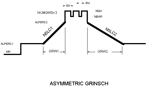
Error Messages
File system errors
33 - directory full
34 - disk full
35 - no such volume
36 - I/O error
37 - bad file name
38 - file not open
39 - end of file
40 - tried to position to before start of file
41 - memory full or file wont fit
42 - too many open files
43 - file not found
44 - diskette is write protected
45 - file is locked
46 - volume is locked
47 - file si busy
48 - duplicate filename
49 - file already open
50 - error in user parameter list
51 - invalid file reference number
52 - get file position error
53 - volume not on line error
54 - permissions error
55 - drive volume already on-line
56 - no such drive
57 - not a Mac diskette
58 - volume in question belongs to an external fs
59 - file system error during rename
60 - bad master directory block
61 - write permissions error
Runtine error codes
64 - insufficient memory
65 - numeric overflow
66 - divide by zero
67 - argument error
68 - stack underflow
69 - stack overflow
70 - COMMON buffer not found
71 - illegal record length
72 - record overflow
73 - duplicate virtual array
74 - virtual buffer not found
75 - subprogram not found
76 - FORMAT syntax error
77 - file not open for WRITE
78 - file not open for READ
79 - SELECT CASE match error
80 - argument list mismatch
81 - FORMAT descriptor error
82 - array boundary error
83 - illegal function call
84 - floating point hardware not found
85 - illegal substring expression