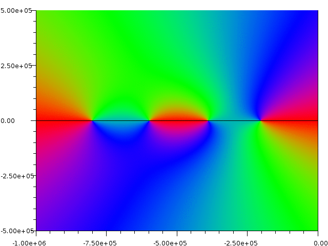
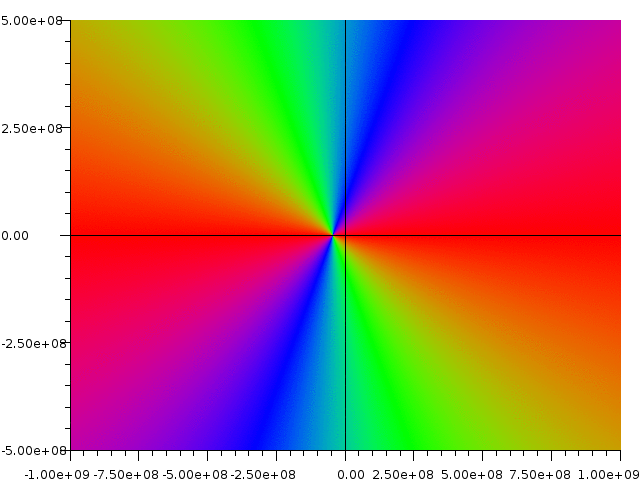
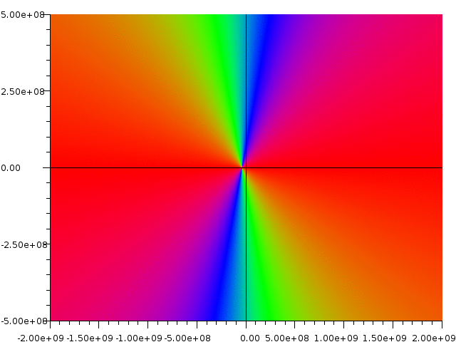
This page presents a new plotting method where the phase of the Laplace transform representing a network transfer function is coded into colors of image pixels. This is a numerically robust plotting method that allows designers to visualize the entire Laplace domain, and see the migration of singular points as a network parameter is varied that is referred to as a "root locus". The singular points are readily apparent with this plotting algorithm. Poles are recognized at points around which the color rapidly spins through red-green-blue in a counterclockwise direction, and zeroes are recognized at points around which the color rapidly spins through red-green-blue in a clockwise direction. For details, see

J. W. Fattaruso, "Visualizing the Laplace Domain", IEEE ISCAS, Montreal, Canada, May 2016
J. W. Fattaruso, "New Graphical Tools for Visualizing the Laplace and z-Domains", IEEE Circuits and Systems Magazine, 3rd Quarter 2017

These example Java applications to generate root locus plots interactively may be freely downloaded, along with example project files that demonstrate each simulator's function. All processor cores available on the hardware these programs are run on are used in a parallel multithreaded fashion to compute the plot images as quickly as possible.

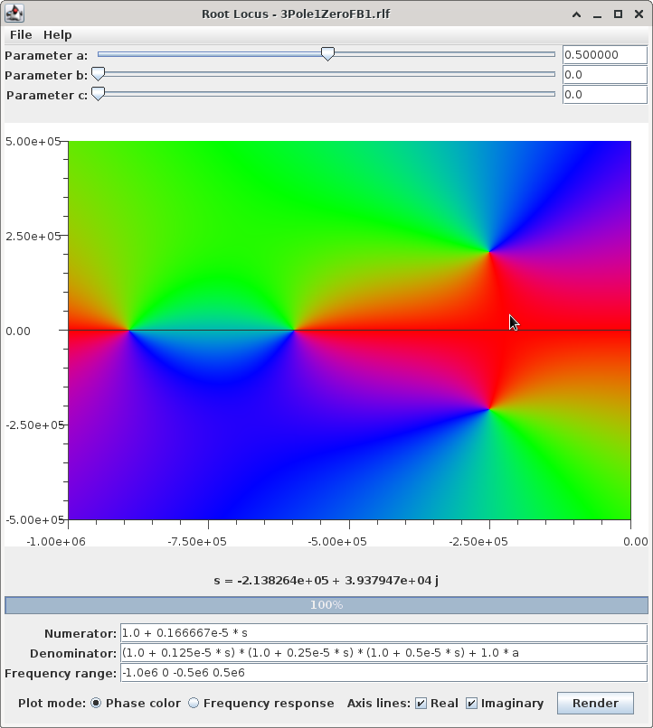
Download the Java application and the example function description files for a 3-pole, 1-zero feedback loop, a 3-pole lowpass filter that can be adjusted from Butterworth to Chebyshev, and a similar 5-pole lowpass filter. In either a Windows Command Prompt window or a Linux terminal emulation window, run the application with the command line

java -jar RootLocusFunction.jar

and use the 'File' menu to open the description file. This will fill out the text input fields in the application with the two complex-valued algebraic expressions representing the numerator and denominator of the rational transfer function. This function of the complex frequency 's' represents the transfer function of the closed loop gain for a forward amplifier with three poles and zero surrounded in a feedback loop. Press the 'Render' button to see the color-coded plot of the Laplace transform. A second plot mode that shows the sinusoidal steady state frequency magnitude (in dB) and phase response is also available.

The third text field is the complex frequency range over which values of the complex frequency variable 's' will be spread to iteratively evaluation the transfer function ratio and fill in the image pixels with phase coded colors. The first two values are the minimum and maximum real component, respectively, in radians/second, and the second two values are the minimum and maximum imaginary component, respectively.

The complex frequency that corresponds to the current mouse pointer position is displayed just under the plot image. The left mouse button may be used to zoom into a small area of interest in the plot. Click and drag a rectangle to temporarily narrow the frequence range. The 'Render' button will reset the area back to that specified in the text field.

Note the presence of the parameter 'a' in the expression for the denominator, representing the feedback factor. This is a real-valued free parameter that may be adjusted by the top slider above the plotting area to observe the locus of singular points that develop as the feedback factor is varied. (It may take your computer a few seconds to recalculate the image each time the slider is moved.)

You may edit the text fields to enter whatever transfer function you would like to analyze and save the description in a file. The saved file format is very simple, and is just the contents of the three text fields on separate lines in a text file. Any of the three free parameters 'a', 'b' and 'c' may be included in the expressions. The sliders along the top can be used to adjust any of the parameters over a range of 0 to 1.

Included in the algebraic expressions for numerator and denominator may be calls to the functions conj(), recip(), exp(), sin(), cos(), tan(), sqrt(),mag(),phase(), real(), imag() and complex(). The complex() function takes two real arguments for the real and imaginary components and returns a complex value. Note that the constant 'j' in engineering Laplace transform expressions (the square root of -1) may therefore be written in this tool as complex(0,1).

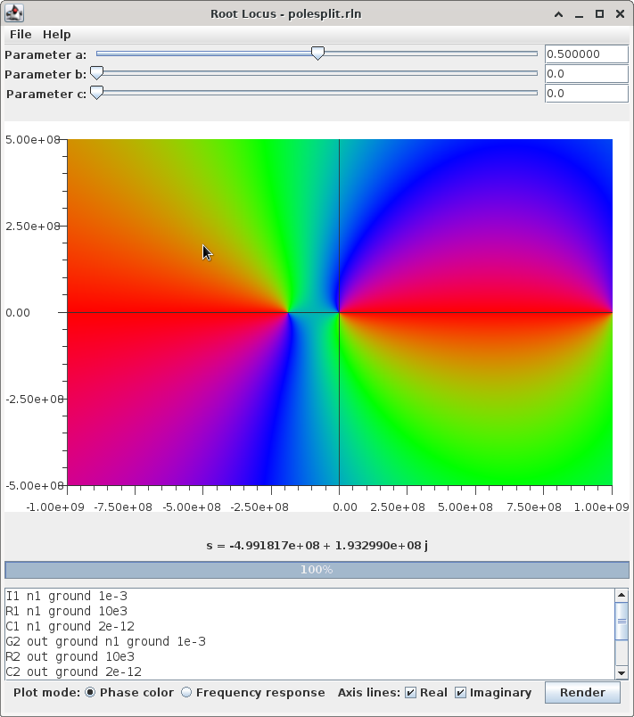
Download the Java application and the example netlist files for a two-stage pole split opamp, a 7th order Butterworth low pass filter, a 7th order Butterworth high pass filter, a 7th order Chebyshev low pass filter, a Colpitts oscillator, and a Hartley oscillator. Run the application with the command line

java -jar RootLocusNetwork.jar

and use the 'File' menu to open a netlist file. The first example file will fill out the text input area in the application with a netlist representing a two stage amplifier with a pole-splitting compensation capacitor. Press the 'Render' button to see the color-coded plot of the Laplace transform. A second plot mode that shows the sinusoidal steady state frequency magnitude (in dB) and phase response is also available.

The lines in the netlist represent network circuit elements or simulation control. The possible circuit elements that are recognized are:

R<name> <node1> <node2> <value>
C<name> <node1> <node2> <value>
L<name> <node1> <node2> <value>
I<name> <node1> <node2> <value>
g<name> <node1> <node2> <node3> <node4> <value>

and represent resistors, capacitors, inductors, independent current sources, and voltage controlled current sources, respectively, in the usual SPICE-like input format. The netlist parser is insensitive to character case, and lines may be commented out with an '*' as the first character. For this netlist parser the <value> field, representing the resistance, capacitance, inductance, current amplitude or source dependence factor, must be either a constant in standard floating point constant format or an algebraic expression in one of the three free parameters. No special SPICE 'scale factors' such as a trailing 'k' or 'm' or 'u' character is recognized here. Node names may be any alphanumeric name desired, but the datum node must be named 'ground', not '0'. There must be at least one independent current source with a unity value that forms the Laplace transform of the input to the network. Note that this simulator performs a simple nodal analysis of the network, so only current sources are allowed.

Two simulation control lines must be included at the end of the netlist. One is of the form

.plot <node>

and informs the simulator which node in the network is considered the output node for the transfer function. The second required control line is of the form

.freq <real min> <real max> <imag min> <imag max>

This statement specifies the range of the real and imaginary components of the complex frequency variable 's' over which the Laplace transform will be evaluated.

The complex frequency that corresponds to the current mouse pointer position is displayed just under the plot image. The left mouse button may be used to zoom into a small area of interest in the plot. Click and drag a rectangle to temporarily narrow the frequence range. The 'Render' button will reset the area back to that specified in the '.freq' line.

As mentioned above, any element value on any of the element lines may optionally consist of an algebraic expression enclosed in parentheses '()'. In these expressions may appear any of the free parameters 'a', 'b' and 'c'. These parameters may be adjusted in real time with the sliders along the top of the application window, and the root locus of the transfer function developed in the plotting area. (It may take your computer a few seconds to recalculate the image each time the slider is moved.) The parameter 'a' in the example two stage amplifier netlist controls the value of the compensation capacitance CC.

You may edit the text area to enter whatever netlist you would like to simulate and save the netlist in a file. The saved file format is very simple, and is just the contents of the text area in a plain text file.

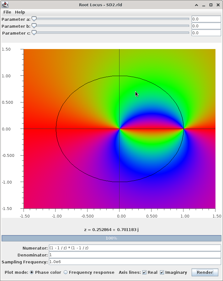
Download the Java application and the example discrete function description files for a first order sigma-delta modulator, a second order sigma-delta modulator, and a 5th order Butterworth low pass filter. In either a Windows Command Prompt window or a Linux terminal emulation window, run the application with the command line

java -jar RootLocusDiscrete.jar

and use the 'File' menu to open the description file. This will fill out the text input fields in the application with the two complex-valued algebraic expressions representing the numerator and denominator of the rational discrete time transfer function and the sample rate in Hz. This function of the complex frequency 'z' represents the discrete time quantization noise transfer function of each modulator. Press the 'Render' button to see the color-coded plot of the z-transform. A second plot mode that shows the sinusoidal steady state frequency magnitude (in dB) and phase response is also available.

These programs are distributed "as-is" in the hope that they will be useful, but WITHOUT ANY WARRANTY; without even the implied warranty of MERCHANTABILITY or FITNESS FOR A PARTICULAR PURPOSE. IN NO EVENT SHALL THE AUTHOR BE LIABLE FOR ANY DIRECT, INDIRECT, INCIDENTAL, SPECIAL, EXEMPLARY, OR CONSEQUENTIAL DAMAGES (INCLUDING, BUT NOT LIMITED TO, PROCUREMENT OF SUBSTITUTE GOODS OR SERVICES; LOSS OF USE, DATA, OR PROFITS; OR BUSINESS INTERRUPTION) HOWEVER CAUSED AND ON ANY THEORY OF LIABILITY, WHETHER IN CONTRACT, STRICT LIABILITY, OR TORT (INCLUDING NEGLIGENCE OR OTHERWISE) ARISING IN ANY WAY OUT OF THE USE OF THIS SOFTWARE, EVEN IF ADVISED OF THE POSSIBILITY OF SUCH DAMAGE.

Back to John Fattaruso's home page