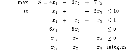
The optimal LP solution is ![]() . Since each variable could be rounded either up or down, there are eight possible ways of rounding the optimal LP solution to get an integer-valued solution.
Unfortunately, all eight ways lead to infeasible solutions.
. Since each variable could be rounded either up or down, there are eight possible ways of rounding the optimal LP solution to get an integer-valued solution.
Unfortunately, all eight ways lead to infeasible solutions.
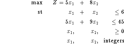

Integer Linear Programming
A linear program with the added restriction that the decision variables must have integer variables is called an integer linear program (ILP) or simply an integer program (IP).
One approach to solving integer programs is to ignore or relax the integer restriction and solve the resulting LP. For some types of problems, for example minimum cost network flow problems, there will always be an optimal LP solution that is also an integer-valued solutions. Such a solution must also be the optimal IP solution. This will not work for ``most'' integer programs, however, because the optimal LP solution may contain variables with non-integer values. When this happens, it might be possible to round the values of LP solution up or down to get an integer-valued solution. For the reasons outlined below, this technique does work very often.

The optimal LP solution is ![]() . Since each variable could be rounded either up or down, there are eight possible ways of rounding the optimal LP solution to get an integer-valued solution.
Unfortunately, all eight ways lead to infeasible solutions.
. Since each variable could be rounded either up or down, there are eight possible ways of rounding the optimal LP solution to get an integer-valued solution.
Unfortunately, all eight ways lead to infeasible solutions.


An LP-Based Branch-and-Bound Algorithm for Integer Programming
Consider the following binary integer program (BIP). A binary variable is one that is constrained to be either 1 or 0.

In this case, we create the LP relaxation by replacing the binary constraints with constraints of the form ![]() . The LP relaxation and optimal solution (obtained with CPLEX) are shown below.
. The LP relaxation and optimal solution (obtained with CPLEX) are shown below.
Maximize
 obj: 75 x1 + 6 x2 + 3 x3 + 33 x4
Subject To
 c1: 774 x1 + 76 x2 + 22 x3 + 42 x4 <= 875
 c2: 67 x1 + 27 x2 + 794 x3 + 53 x4 <= 875
Bounds
 0 <= x1 <= 1
 0 <= x2 <= 1
 0 <= x3 <= 1
 0 <= x4 <= 1


Primal - Optimal:  Objective =    1.1383727197e+02
Solution time =    0.00 sec.    Iterations = 4 (0)


Variable Name           Solution Value
x1                            1.000000
x2                            0.506042
x3                            0.933674
x4                            1.000000
Although solving the LP relaxation did not give us an integer solution, it does give us some information. For example, we know that the best integer solution, if there is one, has an objective function value of at most 113. This is because any integer solution is also a solution to the LP relaxation and therefore cannot have an objective function of more than 113.84. Since all the objective function coefficients are integer-valued, we know that an integer solution could have an objective function of at most 113.
In the optimal LP
relaxation, there are two variables that do not have integer
variables: ![]() and
and ![]() . Since
. Since ![]() two must be either 0 or 1
in a feasible solution to the original BIP, we will create and solve
two new problems, called subproblems by adding constraints to
the LP relaxation.
two must be either 0 or 1
in a feasible solution to the original BIP, we will create and solve
two new problems, called subproblems by adding constraints to
the LP relaxation.
For the case where ![]() , we create subproblem 1 by adding the
constraint
, we create subproblem 1 by adding the
constraint ![]() and solving the resulting problem with CPLEX.
and solving the resulting problem with CPLEX.
Maximize
 obj: 75 x1 + 6 x2 + 3 x3 + 33 x4
Subject To
 c1: 774 x1 + 76 x2 + 22 x3 + 42 x4 <= 875
 c2: 67 x1 + 27 x2 + 794 x3 + 53 x4 <= 875
 c3: x2  = 0
Bounds
 0 <= x1 <= 1
 0 <= x2 <= 1
 0 <= x3 <= 1
 0 <= x4 <= 1

Primal - Optimal:  Objective =    1.1085264484e+02

Variable Name           Solution Value
x1                            1.000000
x3                            0.950882
x4                            1.000000
All other variables in the range 1-4 are zero.
For the case where ![]() , we create subproblem 2 by adding the
constraint
, we create subproblem 2 by adding the
constraint ![]() and solving the resulting problem with CPLEX.
and solving the resulting problem with CPLEX.
Maximize
 obj: 75 x1 + 6 x2 + 3 x3 + 33 x4
Subject To
 c1: 774 x1 + 76 x2 + 22 x3 + 42 x4 <= 875
 c2: 67 x1 + 27 x2 + 794 x3 + 53 x4 <= 875
 c3: x2  = 1
Bounds
 0 <= x1 <= 1
 0 <= x2 <= 1
 0 <= x3 <= 1
 0 <= x4 <= 1

Primal - Optimal:  Objective =    1.1315228795e+02

Variable Name           Solution Value
x1                            0.951860
x2                            1.000000
x3                            0.920939
x4                            1.000000
We still haven't found a feasible BIP solution, but we do know that if ![]() , the best possible objective function value is 110 and that if
, the best possible objective function value is 110 and that if ![]() , the best possible objective function value is 113.
, the best possible objective function value is 113.
Going back to subproblem 1, we create subproblem 3 by adding the constraint ![]() and subproblem 4 by adding the constraint
and subproblem 4 by adding the constraint ![]() .
.
Here are the results for subproblem 3.
Maximize
 obj: 75 x1 + 6 x2 + 3 x3 + 33 x4
Subject To
 c1: 774 x1 + 76 x2 + 22 x3 + 42 x4 <= 875
 c2: 67 x1 + 27 x2 + 794 x3 + 53 x4 <= 875
 c3: x2  = 0
 c4: x3  = 0
Bounds
 0 <= x1 <= 1
 0 <= x2 <= 1
 0 <= x3 <= 1
 0 <= x4 <= 1

Primal - Optimal:  Objective =    1.0800000000e+02

Variable Name           Solution Value
x1                            1.000000
x4                            1.000000
All other variables in the range 1-4 are zero.
We have just found our first feasible BIP solution. Let ![]() be the objective function value of the best BIP solution, called the incumbent solution, found so far. In this case,
be the objective function value of the best BIP solution, called the incumbent solution, found so far. In this case, ![]() and the incumbent solution is
and the incumbent solution is ![]() ,
, ![]() ,
, ![]() and
and ![]() .
.
Here are the results for subproblem 4.
Maximize
 obj: 75 x1 + 6 x2 + 3 x3 + 33 x4
Subject To
 c1: 774 x1 + 76 x2 + 22 x3 + 42 x4 <= 875
 c2: 67 x1 + 27 x2 + 794 x3 + 53 x4 <= 875
 c3: x2  = 0
 c4: x3  = 1
Bounds
 0 <= x1 <= 1
 0 <= x2 <= 1
 0 <= x3 <= 1
 0 <= x4 <= 1

Primal - Optimal:  Objective =    8.6716981132e+01

Variable Name           Solution Value
x1                            1.000000
x3                            1.000000
x4                            0.264151
All other variables in the range 1-4 are zero.
Notice that the objective function value of subproblem 4 is less than
![]() . This means that we do not need to consider creating new
subproblem by adding constraints to subproblem 4 because any BIP
solutions they could generated would have worse objective function
value than our incumbent solution. Also, there is no point in
creating subproblems by adding constraints to subproblem 3 because
its solution is already integer-valued and adding additional
constraints could make the solution worse. So, we know that of all
the solutions where BIP solutions where
. This means that we do not need to consider creating new
subproblem by adding constraints to subproblem 4 because any BIP
solutions they could generated would have worse objective function
value than our incumbent solution. Also, there is no point in
creating subproblems by adding constraints to subproblem 3 because
its solution is already integer-valued and adding additional
constraints could make the solution worse. So, we know that of all
the solutions where BIP solutions where ![]() (half of the 16
possible solutions), the best possible objective function value is 108.
(half of the 16
possible solutions), the best possible objective function value is 108.
Now, we go back to subproblem 2 and create subproblems 5 and 6 by
adding the constraint that ![]() or
or ![]() . Notice that we could
also have created subproblems by constraining
. Notice that we could
also have created subproblems by constraining ![]() to be either 0 or
1.
to be either 0 or
1.
Here are the results for subproblem 5.
Maximize
 obj: 75 x1 + 6 x2 + 3 x3 + 33 x4
Subject To
 c1: 774 x1 + 76 x2 + 22 x3 + 42 x4 <= 875
 c2: 67 x1 + 27 x2 + 794 x3 + 53 x4 <= 875
 c3: x2  = 1
 c4: x1  = 0
Bounds
 0 <= x1 <= 1
 0 <= x2 <= 1
 0 <= x3 <= 1
 0 <= x4 <= 1

Primal - Optimal:  Objective =    4.2000000000e+01

Variable Name           Solution Value
x2                            1.000000
x3                            1.000000
x4                            1.000000
All other variables in the range 1-4 are zero.
This gives us an integer-valued solution, but it is not as good as the incumbent solution.
Here are the results for subproblem 6.
Maximize
 obj: 75 x1 + 6 x2 + 3 x3 + 33 x4
Subject To
 c1: 774 x1 + 76 x2 + 22 x3 + 42 x4 <= 875
 c2: 67 x1 + 27 x2 + 794 x3 + 53 x4 <= 875
 c3: x2  = 1
 c4: x1  = 1
Bounds
 0 <= x1 <= 1
 0 <= x2 <= 1
 0 <= x3 <= 1
 0 <= x4 <= 1

Primal - Optimal:  Objective =    1.0064285714e+02

Variable Name           Solution Value
x1                            1.000000
x2                            1.000000
x4                            0.595238
All other variables in the range 1-4 are zero.
Notice that the objective function value of subproblem 6 is 100.64
which is less than ![]() . This means that we do not need to
consider creating new subproblems by adding constraints to subproblem 6
because any BIP solutions they could generated would have worse
objective function values than our incumbent solution. Also, there is
no point in creating subproblems by adding constraints to subproblem 5
because its solution is already integer-valued and adding additional
constraints could make the solution worse. So, we know that none of
the solutions where BIP solutions where
. This means that we do not need to
consider creating new subproblems by adding constraints to subproblem 6
because any BIP solutions they could generated would have worse
objective function values than our incumbent solution. Also, there is
no point in creating subproblems by adding constraints to subproblem 5
because its solution is already integer-valued and adding additional
constraints could make the solution worse. So, we know that none of
the solutions where BIP solutions where ![]() have an objective
function value of more than 108. Thus our incumbent solution is an
optimal BIP solution.
have an objective
function value of more than 108. Thus our incumbent solution is an
optimal BIP solution.
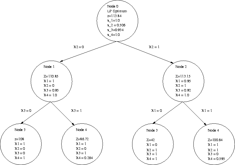
The process followed above, know as the branch-and-bound algorithm can be presented graphically as shown below.
Summary of the Generic Branch-and-Bound Technique for Maximization IP's
If the optimal solution to the LP relaxation is integer-valued, then it is also an optimal IP solution and we can stop. Otherwise, the LP relaxation becomes the first unfathomed node of the branch-and-bound tree. Let Z, the optimal objective function of the LP relaxation, be the bound on the the first unfathomed node
Find the bound for each of the two new nodes of the branch-and-bound tree by solving the associated subproblems (LP's) and letting the Z values (the optimal objective function values) be the bounds.
Let Z be the bound for a new node. The node becomes fathomed (discarded) if any of the following conditions are true.
If there are no more unfathomed nodes in the branch-and-bound tree and there is an incumbent solution, then the incumbent solution is optimal. If there are no more unfathomed nodes in the branch-and-bound tree and there is no incumbent solution, then the problem has no feasible solution. Otherwise, return to the Branching Step.