OR MODELS Blending and Production-Process Problems

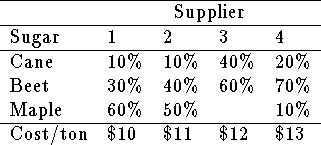
Blending: (Based on problem 2-3 from AMPL book page 35): A soft-drink manufacturer wishes to blend three types of sugar in approximately equal quantities to ensure a uniformity of taste in a product. Sugar suppliers only provide combinations (mixtures) of the sugars at varying costs per ton:

Formulate an LP model that minimizes the cost of supply while producing a blend that contains 16 tons of cane sugar, 44 tons of corn sugar and 40 tons of beet sugar.

Solution

• Let be the number of tons purchased from supplier i = 1, 2, 3, 4.
• Let be the tons of sugar of type j = c, b, m.

Objective Function:

Constraints:

Required tons of each type of sugar

• One ton from supplier 1 has 0.1 tons of cane sugar, 0.3 tons of beet sugar and 0.6 tons of maple sugar.
• One ton from supplier 2 has 0.1 tons of cane sugar, 0.4 tons of beet sugar and 0.5 tons of maple sugar.
• From the proportionality and additivity assumptions, mixing one ton from supplier 1 with one ton from supplier 2 gives a mixture with 0.2 tons of cane sugar, 0.7 tons of beet sugar 1.1 tons of maple sugar.

Blending Constraints

LP formulation in CPLEX format

minimize 10 x1 + 11 x2 + 12 x3 + 13 x4
subject to
yc - 0.1 x1 - 0.1 x2 - 0.4 x3 - 0.2 x4 = 0
yb - 0.3 x1 - 0.4 x2 - 0.6 x3 - 0.7 x4 = 0
ym - 0.6 x1 - 0.5 x2 - 0.0 x3 - 0.1 x4 = 0
yc = 16
yb = 44
ym = 40
end

Optimal Solution

Primal - Optimal:  Objective =    1.1022222222e+03
Solution time =    0.00 sec.  Iterations = 1 (0)

Variable Name           Solution Value
x1                           62.222222
x3                           11.111111
x4                           26.666667
yc                           16.000000
yb                           44.000000
ym                           40.000000
All other variables in the range 1-7 are zero.

Alternative Problem Statement: Formulate an LP to minimize the cost of producing one ton of blend that is 16% cane sugar, 44% beet sugar and 40% maple sugar.

Solution

LP formulation in CPLEX format

minimize 10 x1 + 11 x2 + 12 x3 + 13 x4
subject to
yc - 0.1 x1 - 0.1 x2 - 0.4 x3 - 0.2 x4 = 0
yb - 0.3 x1 - 0.4 x2 - 0.6 x3 - 0.7 x4 = 0
ym - 0.6 x1 - 0.5 x2 - 0.0 x3 - 0.1 x4 = 0
yc - 0.16 yc - 0.16 yb - 0.16 ym = 0
yb - 0.44 yc - 0.44 yb - 0.44 ym = 0
ym - 0.40 yc - 0.40 yb - 0.40 ym = 0
yc + yb + ym = 1
end

Optimal Solution

Primal - Optimal:  Objective =    1.1022222222e+01

Variable Name           Solution Value
x1                            0.622222
x3                            0.111111
x4                            0.266667
yc                            0.160000
yb                            0.440000
ym                            0.400000
All other variables in the range 1-7 are zero.

Formulate an LP to minimize the cost of producing one ton of blend that is 20% cane sugar, 50% beet sugar and 30% maple sugar.

LP formulation in CPLEX format

minimize 10 x1 + 11 x2 + 12 x3 + 13 x4
subject to
yc - 0.1 x1 - 0.1 x2 - 0.4 x3 - 0.2 x4 = 0
yb - 0.3 x1 - 0.4 x2 - 0.6 x3 - 0.7 x4 = 0
ym - 0.6 x1 - 0.5 x2 - 0.0 x3 - 0.1 x4 = 0
yc - 0.2 yc - 0.2 yb - 0.2 ym = 0
yb - 0.5 yc - 0.5 yb - 0.5 ym = 0
ym - 0.3 yc - 0.3 yb - 0.3 ym = 0
yc + yb + ym = 1
end

Optimal Solution

Primal - Optimal:  Objective =    1.1444444444e+01
Solution time =    0.00 sec.  Iterations = 0 (0)


Variable Name           Solution Value
x1                            0.444444
x3                            0.222222
x4                            0.333333
yc                            0.200000
yb                            0.500000
ym                            0.300000
All other variables in the range 1-7 are zero.

A Two-Product Blending Problem: Formulate an LP to maximize profit for two products.

• Product 1:
  • Requires a blend that is 16% cane sugar, 44% beet sugar and 40% maple sugar.
  • Sells for $20/ton
• Product 2:
  • Requires a blend that is 25% cane sugar, 45% beet sugar and 30% maple sugar.
  • Sells for $25/ton
• At most 5 tons of sugar mixture may be purchased from any one supplier.
• Supplier data from the first example applies.

Solution

• Let be the tons of mixture from supplier i used to produce product k.
• Let be the tons of sugar type j in product k.
• Let be the tons of product j produced.
• Maximize profit = revenue - cost =

  

LP formulation in CPLEX format

maximize 20 p1 + 25 p2 -
 10 x11 - 10 x12 - 11 x21 - 11 x22 - 12 x31 - 12 x32 - 13 x41 - 13 x42
subject to
yc1 - 0.1 x11 - 0.1 x21 - 0.4 x31 - 0.2 x41 = 0
yb1 - 0.3 x11 - 0.4 x21 - 0.6 x31 - 0.7 x41 = 0
ym1 - 0.6 x11 - 0.5 x21 - 0.0 x31 - 0.1 x41 = 0
yc1 - 0.16 yc1 - 0.16 yb1 - 0.16 ym1 = 0
yb1 - 0.44 yc1 - 0.44 yb1 - 0.44 ym1 = 0
ym1 - 0.40 yc1 - 0.40 yb1 - 0.40 ym1 = 0
yc2 - 0.1 x12 - 0.1 x22 - 0.4 x32 - 0.2 x42 = 0
yb2 - 0.3 x12 - 0.4 x22 - 0.6 x32 - 0.7 x42 = 0
ym2 - 0.6 x12 - 0.5 x22 - 0.0 x32 - 0.1 x42 = 0
yc2 - 0.25 yc2 - 0.25 yb2 - 0.25 ym2 = 0
yb2 - 0.45 yc2 - 0.45 yb2 - 0.45 ym2 = 0
ym2 - 0.3 yc2 - 0.3 yb2 - 0.3 ym2 = 0
x11 + x12 <= 5
x21 + x22 <= 5
x31 + x32 <= 5
x41 + x42 <= 5
p1 - x11 - x21 - x31 - x41 = 0
p2 - x12 - x22 - x32 - x42 = 0
end

Optimal Solution

Primal - Optimal:  Objective =    1.7434782609e+02

CPLEX> dis sol -
Variable Name           Solution Value
p1                            8.695652
p2                            6.956522
x11                           1.521739
x12                           3.478261
x21                           5.000000
x31                           1.521739
x32                           3.478261
x41                           0.652174
yc1                           1.391304
yb1                           3.826087
ym1                           3.478261
yc2                           1.739130
yb2                           3.130435
ym2                           2.086957
All other variables in the range 1-16 are zero.

A Production Process Model: A farmer has 45 acres on which she can plant wheat or corn. To plant an acre of wheat, the farmer requires 3 labor-hours and 2 tons of fertilizer. To plant an acre of corn, the farmer requires 2 labor-hours and 4 tons of fertilizer. The farmer has 100 labor-hours and 120 tons of fertilizer available. The profits for harvesting and selling an acre of wheat and corn are $200 and $300, respectively. The harvested wheat and corn can either be sold as is or it can be further processed to produce premium wheat and corn.

Processing one and one half acres of a crop requires two labor-hours and yields one acre's worth of the premium crop. One acre's worth of premium wheat sells for $350 and one acre's worth of premium corn sells for $450.

Formulate an LP which can be used to determine how much each crop should be planted, how much be should sold as is and how much should be further processed and sold as the premium variety.

Solution

• Let aw be the number of acres of wheat planted
• Let ac be the number of acres of corn planted
• Let w be the number of acres of regular wheat sold.
• Let pw be the number of acres of premium wheat sold.
• Let c be the number of acres of regular corn sold.
• Let pc be the number of acres of premium corn sold.

LP formulation in CPLEX format

max  200 w + 300 c + 350 pw + 450 pc
s.t. 
3 aw + 2 ac + 2 pw + 2 pc <= 100
2 aw + 4 ac <= 120
aw + ac <= 45
w + 1.5 pw - aw <= 0
c + 1.5 pc - ac <= 0
end

Optimal Solution

Primal - Optimal:  Objective =    1.0000000000e+04
Variable Name           Solution Value
c                            24.000000
pw                            8.000000
aw                           12.000000
ac                           24.000000
All other variables in the range 1-6 are zero.

Multiperiod Financial Models

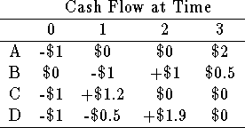
Problem: Determine an optimal investment strategy for the next three years given that:

• $150,000 available at time 0.
• At most, $50,000 may be invested in any one investment.
• Money not spent on other investments can be put into money market funds that pay 10% per year.
• Returns from investments may be immediately reinvested.

  For example, positive cash flow from investment C at time 1 may reinvested in investment B.

Solution

• A = dollars invested in investment A
• B = dollars invested in investment B
• C = dollars invested in investment C
• D = dollars invested in investment D
• = dollars invested in money market funds at time t (t = 0, 1, 2)

Example:

Time 0:

Invest $2 in C.

Time 1:

Receive $2 1.2 = $2.4 from C.

Time 1:

Invest $2.4 in B.

Time 2:

Receive $2.4 from B.

Time 2:

Invest $2.4 in the money market fund.

Time 3:

Receive $1.2 from B and $2.4 1.1 = $2.64 from the money market fund. Total cash received = $3.84.

Objective Function: Maximize the cash on hand at time 3.

Constraints:

Initial investment (time 0):

Cash invested at time t = cash on hand at time t

(time 1)

time 2:

Bounds:

LP in CPLEX format:

max 2 A + 0.5 B + 1.1 S2
subject to 
A + C + D + S0 = 150000
1.2 C + 1.1 S0 - B - 0.5 D - S1 = 0
B + 1.9 D + 1.1 S1 - S2 = 0
A <= 50000
B <= 50000
C <= 50000
D <= 50000
end

Optimal Solution

Primal - Optimal:  Objective =    2.6490625000e+05

Variable Name           Solution Value
A                         50000.000000
B                         50000.000000
S2                       127187.500000
C                         50000.000000
D                         40625.000000
S0                         9375.000000
All other variables in the range 1-7 are zero.

Interpretation

Time 0

Invest $50,000 in A and C, $40,625 in D and $9,375 in the money market fund.

$50,000 + $50,000 + $40,625 + $9,375 = $150,000.

Time 1

Receive:

• $9,375 1.1 = $10,312.5 from the money market fund
• $50,000 1.2 = $60,000 from investment C
• Total cash received = $70,312.5

Invest:

• $40,625 0.5 = $20,312.5 in D
• $50,000 in B.
• Total investment = $70,312.5.

Time 2

Receive

• $50,000 from B
• $40,625 1.9 = 77,187.5 from D
• Total cash received = $127,187.5

Invest 127,187.5 in the money market fund.

Time 3

Receive

• $100,000 from A
• $25,000 from B
• $127187.5 1.1 = $139,906.25
• Total cash received = $264,906.25

• About this document ...