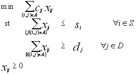
A Transportation Problem is a special case of the MCNFP where there is a set S of n supply nodes, at set D of m demand nodes, no transshipment nodes and no upper bounds on arc flows. Because there are no transshipment nodes or upper bounds on arc flow, the MCNFP LP formulation for the transportation problem simplified to

If the total demand is greater than the total supply, then problem is infeasible. If the total demand is equal to the total supply, the problem is said to be a balanced transportation problem. If the total supply is greater than the total demand, we can add a dummy demand node to create a balanced problem.

The lp formulation for a balanced transportation problem is

The constraint matrix for a balanced transportation problem has a special structure for which researchers have developed more efficient special-purpose variants of the Simplex method.
 
 

GT Railroad has locomotives at IE Junction, Centerville and Wayover City and needs to get locomotives to the following destinations: A-Station, Fine Place, Goodville and Somewhere Street. A single locomotive is required at each destination. Currently there are four locomotives at IE Junction, one at Centerville, and two at Wayover City. GT Railroad can send a locomotive from any of the three origin locations (IE Junction, Centerville and Wayover City) to any of the destinations. For example, they could send one locomotive to each destination from IE Junction. The goal, however, is to minimize the total distance that the locomotives are sent. This may be because the cost of sending a locomotive from one place to another is directly proportional to the distance traveled. The distances between the origins and destinations are given in the following table.
 
 
 
 
 
 
 

	A-Station	Fine Place	Goodville	Somewhere Street
IE Junction	13	35	42	9
Centerville	6	61	18	30
Wayover City	15	10	5	9

 
 
 

Formulation as a Transportation Problem

1. There are three supply nodes: IE Junction, Centerville and Wayover. Let s1 = 4 be the supply at IE Junction, s2 = 1 be the supply at Centerville and s3 =2 be the supply at Wayover City.
2. Let A-Station be demand node 1, Fine Place demand node 2, Goodville be demand node 3 and Somewhere Street demand node 4. Since a single locomotive is needed at each demand point, di = 1 for i = 1,2,3 and 4.
3. The cost cij of shipping one unit from supply node i to demand node j is the distance from the supply point to the demand point given in the table above.

Minimize 13 X11 + 35 X12 + 42 X13 + 9 X14 + 6 X21 + 61 X22 + 18 X23 + 30 X24 + 15 X31 + 10 X32 + 5 X33 + 9 X34
 
 

Subject to

X11 + X12 + X13 + X14 <= 4 Supply at IE Junction

X21 + X22 + X23 + X24 <= 1 Supply at Centerville

X31 + X32 + X33 + X34 <= 2 Supply at Wayover City

X11 + X21 + X31 >= 1 Demand at A-Station

X12 + X22 + X32 >= 1 Demand at Fine Place

X13 + X23 + X33 >= 1 Demand at Goodville

X14 + X24 + X34 >= 1 Demand at Somewhere Street

Xij >= 0
 
 
 
 

Formulation as a Balanced Transportation Problem

Since total supply is 7 and the total demand is only 4, we add a dummy demand node with a demand d5 = 3. We also add zero-cost arcs from the supply nodes to the dummy node. Thus, the LP formulation changes to:

Minimize 13 X11 + 35 X12 + 42 X13 + 9 X14 + 6 X21 + 61 X22 + 18 X23 + 30 X24 + 15 X31 + 10 X32 + 5 X33 + 9 X34
 
 

Subject to

X11 + X12 + X13 + X14 + X15 = 4 Supply at IE Junction

X21 + X22 + X23 + X24 + X25 = 1 Supply at Centerville

X31 + X32 + X33 + X34 + X35 = 2 Supply at Wayover City

X11 + X21 + X31 = 1 Demand at A-Station

X12 + X22 + X32 = 1 Demand at Fine Place

X13 + X23 + X33 = 1 Demand at Goodville

X14 + X24 + X34 = 1 Demand at Somewhere Street

X15 + X25 + X35 = 3 Demand at Dummy Node

Xij >= 0
 
 

Observe that if we add up the supply constraints we get

(S) X11 + X12 + X13 + ? + X33 + X34 + X35 = 7.

If we add up the first four demand constraints, we get

(D) X11 + X21 + X31 + X12 + X22 + X32 + X14 + X24 + X34 = 4.
 
 

Subtracting (S) from (D) we get X15 + X25 + X35 = 3. Thus, the demand constraint for the dummy node is implied by the other constraints and we can drop it from the formulation. In general, the LP formulation for a balanced transportation problem has the property that any one constraint is implied by the remaining constraints.
 

Theorem: Every BFS for a balanced transportation problem lp is integer-valued.

For many applications, the balanced transportation problem is actually an integer program. As a result of this theorem, however, we can use the Simplex method to solve balanced transportation problems.