Session 13: Introduction to Parallel Programming Concepts

The demise of Moore’s law has been greatly exaggerated? Or has it?

Historically, we have depended on hardware advances to enable faster and larger simulations. In 1965, Gordon Moore observed that the CPU and RAM transistor count about doubled each year. “Moore’s Law” has since been revised to a doubling once every 2 years, with startling accuracy. However physical limits, e.g. power consumption, heat emission, and even the size of the atom, have currently stopped this expansion on individual processors, with speeds that have leveled off since around 2008.

[from Wikipedia – Moore’s Law]

We can performance calculations faster than we can transfer the data! Oh the humanity!

• The overall rate of any computation is determined not just by the processor speed, but also by the ability of the memory system to feed data to it.
• Thanks to Moore’s law, clock rates of high-end processors have increased at roughly 40% per year since the 1970’s.
• However, over that same time interval, RAM access times have improved at roughly 10% per year.
• This growing mismatch between processor speed and RAM latency presents an increasing performance bottleneck, since the CPU spends more and more time idle, waiting on data from RAM.

Let’s go parallelize something!

In addition, many simulations require incredible amounts of memory to achieve high-accuracy solutions (PDE & MD solvers, etc.), which cannot fit on a single computer alone.

The natural solution to these problems is the use of parallel computing:

• Use multiple processors concurrently to solve a problem in less time.
• Use multiple computers to store data for large problems.

Anatomy of a Cluster

A more cost-effective approach to construction of larger parallel computers relies on a network to connect disjoint computers together:

• Each processor only has direct access to its own local memory address space; the same address on different processors refers to different memory locations.
• Processors interact with one another through passing messages.
• Commercial multicomputers typically provide a custom switching network to provide low-latency, high-bandwidth access between processors.
• Commodity clusters are build using commodity computers and switches/LANs.
• Clearly less costly than SMP, but have increased latency/decreased bandwidth between CPUs.
• Construction may be symmetric, asymmetric, or mixed.
• Theoretically extensible to arbitrary processor counts, but software becomes complicated and networking gets expensive.

Parallelism Defined

• Partitioning/Decomposition: the means by which an overall computation is divided into smaller parts, some or all of which may be executed in parallel.

• Tasks: programmer-defined computational subunits determined through the decomposition.

• Concurrency: the degree to which multiple tasks can be executed in parallel at any given time (more is better).

• Granularity: the size of tasks into which a problem is decomposed
  • A decomposition into a large number of small tasks is called fine-grained.
  • A decomposition into a small number of large tasks is called coarse-grained.

• Task-interaction: the tasks that a problem is decomposed into often share input, output, or intermediate data that must be communicated.

• Processes: individual threads of execution. A single processor may execute multiple processes, each of which can operate on multiple tasks.

To Decompose or Not to Decompose

Any decomposition strategy must determine a set of primitive tasks.

Goals:

• Identify as many primitive tasks as possible (increases potential parallelism): prefer at least an order of magnitude more tasks than processors.
• Minimize redundant computations and data storage (efficiency, scalability).
• Want primitive tasks to be roughly equal work (load balancing).
• Want the number of tasks to increase as the problem gets larger (scalability).
• Data decompositions* are approaches that first divide the data into pieces and then determine how to associate computations with each piece of data.
• Functional decompositions* are approaches that first divide the computation into functional parts and then determine how to associate data items with the individual computations.
• After all that analysis… is it worth the time and effort?

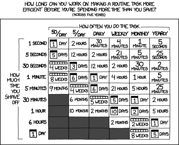
xkcd comic 1205, Is It Worth the Time?