Introduction to Python
Let’s Start with:
export MODULEPATH="${MODULEPATH}:/hpc/modules/workshop"
module --ignore-cache load python_jupyter
cp -R /hpc/examples/workshops/hpc/python-inflammation ~/
cd ~/python-inflammation
srun -p development,htc,mic -c 1 --mem=6G --pty -t 0-2 m2_jupyter_lab
Select the Python 3 install in the Jupyter Lab window.
In this session we will learn how to work with arthritis inflammation datasets in Python. However, before we discuss how to deal with many data points, let’s learn how to work with single data values.
Variables
Any Python interpreter can be used as a calculator:
3 + 5 * 4
23
This is great but not very interesting.
To do anything useful with data, we need to assign its value to a variable.
In Python, we can assign a value to a
variable, using the equals sign =.
For example, to assign value 60 to a variable weight_kg, we would execute:
weight_kg = 60
From now on, whenever we use weight_kg, Python will substitute the value we assigned to
it. In essence, a variable is just a name for a value.
In Python, variable names:
- can include letters, digits, and underscores
- cannot start with a digit
- are case sensitive.
This means that, for example:
weight0is a valid variable name, whereas0weightis notweightandWeightare different variables
Types of data
Python knows various types of data. Three common ones are:
- integer numbers
- floating point numbers, and
- strings.
In the example above, variable weight_kg has an integer value of 60.
To create a variable with a floating point value, we can execute:
weight_kg = 60.0
And to create a string we simply have to add single or double quotes around some text, for example:
weight_kg_text = 'weight in kilograms:'
Using Variables in Python
To display the value of a variable to the screen in Python, we can use the print function:
print(weight_kg)
60.0
We can display multiple things at once using only one print command:
print(weight_kg_text, weight_kg)
weight in kilograms: 60.0
Moreover, we can do arithmetic with variables right inside the print function:
print('weight in pounds:', 2.2 * weight_kg)
weight in pounds: 132.0
The above command, however, did not change the value of weight_kg:
print(weight_kg)
60.0
To change the value of the weight_kg variable, we have to
assign weight_kg a new value using the equals = sign:
weight_kg = 65.0
print('weight in kilograms is now:', weight_kg)
weight in kilograms is now: 65.0
Variables as Sticky Notes
A variable is analogous to a sticky note with a name written on it: assigning a value to a variable is like putting that sticky note on a particular value.
This means that assigning a value to one variable does not change values of other variables. For example, let’s store the subject’s weight in pounds in its own variable:
# There are 2.2 pounds per kilogram
weight_lb = 2.2 * weight_kg
print(weight_kg_text, weight_kg, 'and in pounds:', weight_lb)
weight in kilograms: 65.0 and in pounds: 143.0
Let’s now change
weight_kg:weight_kg = 100.0 print('weight in kilograms is now:', weight_kg, 'and weight in pounds is still:', weight_lb)weight in kilograms is now: 100.0 and weight in pounds is still: 143.0
Since
weight_lbdoesn’t “remember” where its value comes from, it is not updated when we changeweight_kg.


Words are useful, but what’s more useful are the sentences and stories we build with them. Similarly, while a lot of powerful, general tools are built into Python, specialized tools built up from these basic units live in libraries that can be called upon when needed.
Loading data into Python
In order to load our inflammation data, we need to access (import in Python terminology) a library called NumPy which stands for Numerical Python. In general you should use this library if you want to do fancy things with numbers, especially if you have matrices or arrays. We can import NumPy using:
import numpy
Importing a library is like getting a piece of lab equipment out of a storage locker and setting it up on the bench. Libraries provide additional functionality to the basic Python package, much like a new piece of equipment adds functionality to a lab space. Just like in the lab, importing too many libraries can sometimes complicate and slow down your programs - so we only import what we need for each program.
Scientists Dislike Typing
We will always use the syntax
import numpyto import NumPy. However, in order to save typing, it is often suggested to make a shortcut like so:import numpy as np. If you ever see Python code online using a NumPy function withnp(for example,np.loadtxt(...)), it’s because they’ve used this shortcut. When working with other people, it is important to agree on a convention of how common libraries are imported.
Once we’ve imported the library, we can ask the library to read our data file for us:
numpy.loadtxt(fname='inflammation-01.csv', delimiter=',')
array([[ 0.,  0.,  1., ...,  3.,  0.,  0.],
       [ 0.,  1.,  2., ...,  1.,  0.,  1.],
       [ 0.,  1.,  1., ...,  2.,  1.,  1.],
       ...,
       [ 0.,  1.,  1., ...,  1.,  1.,  1.],
       [ 0.,  0.,  0., ...,  0.,  2.,  0.],
       [ 0.,  0.,  1., ...,  1.,  1.,  0.]])
The expression numpy.loadtxt(...) is a function call
that asks Python to run the function loadtxt which
belongs to the numpy library. This dotted notation
is used everywhere in Python: the thing that appears before the dot contains the thing that
appears after.
As an example, John Smith is the John that belongs to the Smith family.
We could use the dot notation to write his name smith.john,
just as loadtxt is a function that belongs to the numpy library.
numpy.loadtxt has two parameters: the name of the file
we want to read and the delimiter that separates values on
a line. These both need to be character strings (or strings
for short), so we put them in quotes.
Since we haven’t told it to do anything else with the function’s output,
the notebook displays it.
In this case,
that output is the data we just loaded.
By default,
only a few rows and columns are shown
(with ... to omit elements when displaying big arrays).
To save space,
Python displays numbers as 1. instead of 1.0
when there’s nothing interesting after the decimal point.
Our call to numpy.loadtxt read our file
but didn’t save the data in memory.
To do that,
we need to assign the array to a variable. Just as we can assign a single value to a variable, we
can also assign an array of values to a variable using the same syntax. Let’s re-run
numpy.loadtxt and save the returned data:
data = numpy.loadtxt(fname='inflammation-01.csv', delimiter=',')
This statement doesn’t produce any output because we’ve assigned the output to the variable data.
If we want to check that the data have been loaded,
we can print the variable’s value:
print(data)
[[ 0.  0.  1. ...,  3.  0.  0.]
 [ 0.  1.  2. ...,  1.  0.  1.]
 [ 0.  1.  1. ...,  2.  1.  1.]
 ...,
 [ 0.  1.  1. ...,  1.  1.  1.]
 [ 0.  0.  0. ...,  0.  2.  0.]
 [ 0.  0.  1. ...,  1.  1.  0.]]
Now that the data are in memory,
we can manipulate them.
First,
let’s ask what type of thing data refers to:
print(type(data))
<class 'numpy.ndarray'>
The output tells us that data currently refers to
an N-dimensional array, the functionality for which is provided by the NumPy library.
These data correspond to arthritis patients’ inflammation.
The rows are the individual patients, and the columns
are their daily inflammation measurements.
Data Type
A Numpy array contains one or more elements of the same type. The
typefunction will only tell you that a variable is a NumPy array but won’t tell you the type of thing inside the array. We can find out the type of the data contained in the NumPy array.print(data.dtype)dtype('float64')This tells us that the NumPy array’s elements are floating-point numbers.
With the following command, we can see the array’s shape:
print(data.shape)
(60, 40)
The output tells us that the data array variable contains 60 rows and 40 columns. When we
created the variable data to store our arthritis data, we didn’t just create the array; we also
created information about the array, called members or
attributes. This extra information describes data in the same way an adjective describes a noun.
data.shape is an attribute of data which describes the dimensions of data. We use the same
dotted notation for the attributes of variables that we use for the functions in libraries because
they have the same part-and-whole relationship.
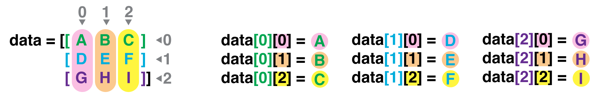
If we want to get a single number from the array, we must provide an index in square brackets after the variable name, just as we do in math when referring to an element of a matrix. Our inflammation data has two dimensions, so we will need to use two indices to refer to one specific value:
print('first value in data:', data[0, 0])
first value in data: 0.0
print('middle value in data:', data[30, 20])
middle value in data: 13.0
The expression data[30, 20] accesses the element at row 30, column 20. While this expression may
not surprise you,
data[0, 0] might.
Programming languages like Fortran, MATLAB and R start counting at 1
because that’s what human beings have done for thousands of years.
Languages in the C family (including C++, Java, Perl, and Python) count from 0
because it represents an offset from the first value in the array (the second
value is offset by one index from the first value). This is closer to the way
that computers represent arrays (if you are interested in the historical
reasons behind counting indices from zero, you can read
Mike Hoye’s blog post).
As a result,
if we have an M×N array in Python,
its indices go from 0 to M-1 on the first axis
and 0 to N-1 on the second.
It takes a bit of getting used to,
but one way to remember the rule is that
the index is how many steps we have to take from the start to get the item we want.
In the Corner
What may also surprise you is that when Python displays an array, it shows the element with index
[0, 0]in the upper left corner rather than the lower left. This is consistent with the way mathematicians draw matrices but different from the Cartesian coordinates. The indices are (row, column) instead of (column, row) for the same reason, which can be confusing when plotting data.
Slicing data
An index like [30, 20] selects a single element of an array,
but we can select whole sections as well.
For example,
we can select the first ten days (columns) of values
for the first four patients (rows) like this:
print(data[0:4, 0:10])
[[ 0.  0.  1.  3.  1.  2.  4.  7.  8.  3.]
 [ 0.  1.  2.  1.  2.  1.  3.  2.  2.  6.]
 [ 0.  1.  1.  3.  3.  2.  6.  2.  5.  9.]
 [ 0.  0.  2.  0.  4.  2.  2.  1.  6.  7.]]
The slice 0:4 means, “Start at index 0 and go up to, but not
including, index 4.”Again, the up-to-but-not-including takes a bit of getting used to, but the
rule is that the difference between the upper and lower bounds is the number of values in the slice.
We don’t have to start slices at 0:
print(data[5:10, 0:10])
[[ 0.  0.  1.  2.  2.  4.  2.  1.  6.  4.]
 [ 0.  0.  2.  2.  4.  2.  2.  5.  5.  8.]
 [ 0.  0.  1.  2.  3.  1.  2.  3.  5.  3.]
 [ 0.  0.  0.  3.  1.  5.  6.  5.  5.  8.]
 [ 0.  1.  1.  2.  1.  3.  5.  3.  5.  8.]]
We also don’t have to include the upper and lower bound on the slice. If we don’t include the lower bound, Python uses 0 by default; if we don’t include the upper, the slice runs to the end of the axis, and if we don’t include either (i.e., if we just use ‘:’ on its own), the slice includes everything:
small = data[:3, 36:]
print('small is:')
print(small)
The above example selects rows 0 through 2 and columns 36 through to the end of the array.
small is:
[[ 2.  3.  0.  0.]
 [ 1.  1.  0.  1.]
 [ 2.  2.  1.  1.]]
Arrays also know how to perform common mathematical operations on their values. The simplest operations with data are arithmetic: addition, subtraction, multiplication, and division. When you do such operations on arrays, the operation is done element-by-element. Thus:
doubledata = data * 2.0
will create a new array doubledata
each element of which is twice the value of the corresponding element in data:
print('original:')
print(data[:3, 36:])
print('doubledata:')
print(doubledata[:3, 36:])
original:
[[ 2.  3.  0.  0.]
 [ 1.  1.  0.  1.]
 [ 2.  2.  1.  1.]]
doubledata:
[[ 4.  6.  0.  0.]
 [ 2.  2.  0.  2.]
 [ 4.  4.  2.  2.]]
If, instead of taking an array and doing arithmetic with a single value (as above), you did the arithmetic operation with another array of the same shape, the operation will be done on corresponding elements of the two arrays. Thus:
tripledata = doubledata + data
will give you an array where tripledata[0,0] will equal doubledata[0,0] plus data[0,0],
and so on for all other elements of the arrays.
print('tripledata:')
print(tripledata[:3, 36:])
tripledata:
[[ 6.  9.  0.  0.]
 [ 3.  3.  0.  3.]
 [ 6.  6.  3.  3.]]
Often, we want to do more than add, subtract, multiply, and divide array elements. NumPy knows how
to do more complex operations, too. If we want to find the average inflammation for all patients on
all days, for example, we can ask NumPy to compute data’s mean value:
print(numpy.mean(data))
6.14875
mean is a function that takes
an array as an argument.
Not All Functions Have Input
Generally, a function uses inputs to produce outputs. However, some functions produce outputs without needing any input. For example, checking the current time doesn’t require any input.
import time
print(time.ctime())
'Sat Mar 26 13:07:33 2016'For functions that don’t take in any arguments, we still need parentheses (
()) to tell Python to go and do something for us.
NumPy has lots of useful functions that take an array as input. Let’s use three of those functions to get some descriptive values about the dataset. We’ll also use multiple assignment, a convenient Python feature that will enable us to do this all in one line.
maxval, minval, stdval = numpy.max(data), numpy.min(data), numpy.std(data)

print('maximum inflammation:', maxval)
print('minimum inflammation:', minval)
print('standard deviation:', stdval)
Here we’ve assigned the return value from numpy.max(data) to the variable maxval, the value
from numpy.min(data) to minval, and so on.
maximum inflammation: 20.0
minimum inflammation: 0.0
standard deviation: 4.61383319712
Mystery Functions in IPython
How did we know what functions NumPy has and how to use them? If you are working in IPython or in a Jupyter Notebook, there is an easy way to find out. If you type the name of something followed by a dot, then you can use tab completion (e.g. type
numpy.and then press tab) to see a list of all functions and attributes that you can use. After selecting one, you can also add a question mark (e.g.numpy.cumprod?), and IPython will return an explanation of the method! This is the same as doinghelp(numpy.cumprod).
When analyzing data, though, we often want to look at variations in statistical values, such as the maximum inflammation per patient or the average inflammation per day. One way to do this is to create a new temporary array of the data we want, then ask it to do the calculation:
patient_0 = data[0, :] # 0 on the first axis (rows), everything on the second (columns)
print('maximum inflammation for patient 0:', numpy.max(patient_0))
maximum inflammation for patient 0: 18.0
Everything in a line of code following the ‘#’ symbol is a comment that is ignored by Python. Comments allow programmers to leave explanatory notes for other programmers or their future selves.
We don’t actually need to store the row in a variable of its own. Instead, we can combine the selection and the function call:
print('maximum inflammation for patient 2:', numpy.max(data[2, :]))
maximum inflammation for patient 2: 19.0
What if we need the maximum inflammation for each patient over all days (as in the next diagram on the left) or the average for each day (as in the diagram on the right)? As the diagram below shows, we want to perform the operation across an axis:
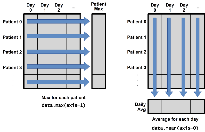
To support this functionality, most array functions allow us to specify the axis we want to work on. If we ask for the average across axis 0 (rows in our 2D example), we get:
print(numpy.mean(data, axis=0))
[  0.           0.45         1.11666667   1.75         2.43333333   3.15
   3.8          3.88333333   5.23333333   5.51666667   5.95         5.9
   8.35         7.73333333   8.36666667   9.5          9.58333333
  10.63333333  11.56666667  12.35        13.25        11.96666667
  11.03333333  10.16666667  10.           8.66666667   9.15         7.25
   7.33333333   6.58333333   6.06666667   5.95         5.11666667   3.6
   3.3          3.56666667   2.48333333   1.5          1.13333333
   0.56666667]
As a quick check, we can ask this array what its shape is:
print(numpy.mean(data, axis=0).shape)
(40,)
The expression (40,) tells us we have an N×1 vector,
so this is the average inflammation per day for all patients.
If we average across axis 1 (columns in our 2D example), we get:
print(numpy.mean(data, axis=1))
[ 5.45   5.425  6.1    5.9    5.55   6.225  5.975  6.65   6.625  6.525
  6.775  5.8    6.225  5.75   5.225  6.3    6.55   5.7    5.85   6.55
  5.775  5.825  6.175  6.1    5.8    6.425  6.05   6.025  6.175  6.55
  6.175  6.35   6.725  6.125  7.075  5.725  5.925  6.15   6.075  5.75
  5.975  5.725  6.3    5.9    6.75   5.925  7.225  6.15   5.95   6.275  5.7
  6.1    6.825  5.975  6.725  5.7    6.25   6.4    7.05   5.9  ]
which is the average inflammation per patient across all days.
##Repeating Actions with Loops
Previously, we wrote Python code that plots values of interest from our first
inflammation dataset (inflammation-01.csv), which revealed some suspicious features in it.

We have a dozen data sets right now, though, and more on the way. We want to create plots for all of our data sets with a single statement. To do that, we’ll have to teach the computer how to repeat things.
An example task that we might want to repeat is printing each character in a word on a line of its own.
word = 'lead'
In Python, a string is just an ordered collection of characters, so every
character has a unique number associated with it – its index. This means that
we can access characters in a string using their indices.
For example, we can get the first character of the word 'lead', by using
word[0]. One way to print each character is to use four print statements:
print(word[0])
print(word[1])
print(word[2])
print(word[3])
l
e
a
d
This is a bad approach for three reasons:
-
Not scalable. Imagine you need to print characters of a string that is hundreds of letters long. It might be easier just to type them in manually.
-
Difficult to maintain. If we want to decorate each printed character with an asterix or any other character, we would have to change four lines of code. While this might not be a problem for short strings, it would definitely be a problem for longer ones.
-
Fragile. If we use it with a word that has more characters than what we initially envisioned, it will only display part of the word’s characters. A shorter string, on the other hand, will cause an error because it will be trying to display part of the string that don’t exist.
word = 'tin'
print(word[0])
print(word[1])
print(word[2])
print(word[3])
t
i
n
---------------------------------------------------------------------------
IndexError                                Traceback (most recent call last)
<ipython-input-3-7974b6cdaf14> in <module>()
      3 print(word[1])
      4 print(word[2])
----> 5 print(word[3])

IndexError: string index out of range
Here’s a better approach:
word = 'lead'
for char in word:
    print(char)
l
e
a
d
This is shorter — certainly shorter than something that prints every character in a hundred-letter string — and more robust as well:
word = 'oxygen'
for char in word:
    print(char)
o
x
y
g
e
n
The improved version uses a for loop to repeat an operation — in this case, printing — once for each thing in a sequence. The general form of a loop is:
for variable in collection:
    # do things using variable, such as print
Using the oxygen example above, the loop might look like this:
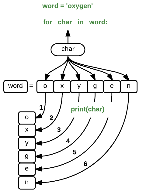
where each character (char) in the variable word is looped through and printed one character
after another. The numbers in the diagram denote which loop cycle the character was printed in (1
being the first loop, and 6 being the final loop).
We can call the loop variable anything we like, but
there must be a colon at the end of the line starting the loop, and we must indent anything we
want to run inside the loop. Unlike many other languages, there is no command to signify the end
of the loop body (e.g. end for); what is indented after the for statement belongs to the loop.
What’s in a name?
In the example above, the loop variable was given the name
charas a mnemonic; it is short for ‘character’. We can choose any name we want for variables. We might just as easily have chosen the namebananafor the loop variable, as long as we use the same name when we invoke the variable inside the loop:word = 'oxygen' for banana in word: print(banana)o x y g e nIt is a good idea to choose variable names that are meaningful, otherwise it would be more difficult to understand what the loop is doing.
Here’s another loop that repeatedly updates a variable:
length = 0
for vowel in 'aeiou':
    length = length + 1
print('There are', length, 'vowels')
There are 5 vowels
It’s worth tracing the execution of this little program step by step.
Since there are five characters in 'aeiou',
the statement on line 3 will be executed five times.
The first time around,
length is zero (the value assigned to it on line 1)
and vowel is 'a'.
The statement adds 1 to the old value of length,
producing 1,
and updates length to refer to that new value.
The next time around,
vowel is 'e' and length is 1,
so length is updated to be 2.
After three more updates,
length is 5;
since there is nothing left in 'aeiou' for Python to process,
the loop finishes
and the print statement on line 4 tells us our final answer.
Note that a loop variable is just a variable that’s being used to record progress in a loop. It still exists after the loop is over, and we can re-use variables previously defined as loop variables as well:
letter = 'z'
for letter in 'abc':
    print(letter)
print('after the loop, letter is', letter)
a
b
c
after the loop, letter is c
Note also that finding the length of a string is such a common operation
that Python actually has a built-in function to do it called len:
print(len('aeiou'))
5
len is much faster than any function we could write ourselves,
and much easier to read than a two-line loop;
it will also give us the length of many other things that we haven’t met yet,
so we should always use it when we can.
From 1 to N
Python has a built-in function called
rangethat generates a sequence of numbers.rangecan accept 1, 2, or 3 parameters.
- If one parameter is given,
rangegenerates a sequence of that length, starting at zero and incrementing by 1. For example,range(3)produces the numbers0, 1, 2.- If two parameters are given,
rangestarts at the first and ends just before the second, incrementing by one. For example,range(2, 5)produces2, 3, 4.- If
rangeis given 3 parameters, it starts at the first one, ends just before the second one, and increments by the third one. For example,range(3, 10, 2)produces3, 5, 7, 9.Using
range, write a loop that usesrangeto print the first 3 natural numbers:1 2 3Solution
for i in range(1, 4):
    print(i)
Understanding the loops
Given the following loop:
word = 'oxygen'
for char in word:
    print(char)
How many times is the body of the loop executed?
- 3 times
- 4 times
- 5 times
- 6 times
Solution
The body of the loop is executed 6 times.
Computing Powers With Loops
Exponentiation is built into Python:
print(5 ** 3)125Write a loop that calculates the same result as
5 ** 3using multiplication (and without exponentiation).Solution
result = 1
for i in range(0, 3):
    result = result * 5
print(result)
Reverse a String
Knowing that two strings can be concatenated using the
+operator, write a loop that takes a string and produces a new string with the characters in reverse order, so'Newton'becomes'notweN'.Solution
newstring = ''
oldstring = 'Newton'
for char in oldstring:
    newstring = char + newstring
print(newstring)
Computing the Value of a Polynomial
The built-in function
enumeratetakes a sequence (e.g. a list) and generates a new sequence of the same length. Each element of the new sequence is a pair composed of the index (0, 1, 2,…) and the value from the original sequence:for i, x in enumerate(xs): # Do something using i and xThe code above loops through
xs, assigning the index toiand the value tox.Suppose you have encoded a polynomial as a list of coefficients in the following way: the first element is the constant term, the second element is the coefficient of the linear term, the third is the coefficient of the quadratic term, etc.
x = 5
cc = [2, 4, 3]
y = cc[0] * x**0 + cc[1] * x**1 + cc[2] * x**2 y = 97Write a loop using
enumerate(cc)which computes the valueyof any polynomial, givenxandcc.Solution
y = 0
for i, c in enumerate(cc):
    y = y + x**i * c
Storing Multiple Values in Lists
Just as a for loop is a way to do operations many times,
a list is a way to store many values.
Unlike NumPy arrays,
lists are built into the language (so we don’t have to load a library
to use them).
We create a list by putting values inside square brackets and separating the values with commas:
odds = [1, 3, 5, 7]
print('odds are:', odds)
odds are: [1, 3, 5, 7]
We can access elements of a list using indices – numbered positions of elements in the list. These positions are numbered starting at 0, so the first element has an index of 0.
print('first element:', odds[0])
print('last element:', odds[3])
print('"-1" element:', odds[-1])
first element: 1
last element: 7
"-1" element: 7
Yes, we can use negative numbers as indices in Python. When we do so, the index -1 gives us the
last element in the list, -2 the second to last, and so on.
Because of this, odds[3] and odds[-1] point to the same element here.
If we loop over a list, the loop variable is assigned to its elements one at a time:
for number in odds:
    print(number)
1
3
5
7
There is one important difference between lists and strings: we can change the values in a list, but we cannot change individual characters in a string. For example:
names = ['Curie', 'Darwing', 'Turing']  # typo in Darwin's name
print('names is originally:', names)
names[1] = 'Darwin'  # correct the name
print('final value of names:', names)
names is originally: ['Curie', 'Darwing', 'Turing']
final value of names: ['Curie', 'Darwin', 'Turing']
works, but:
name = 'Darwin'
name[0] = 'd'
---------------------------------------------------------------------------
TypeError                                 Traceback (most recent call last)
<ipython-input-8-220df48aeb2e> in <module>()
      1 name = 'Darwin'
----> 2 name[0] = 'd'

TypeError: 'str' object does not support item assignment
does not.
Ch-Ch-Ch-Ch-Changes
Data which can be modified in place is called mutable, while data which cannot be modified is called immutable. Strings and numbers are immutable. This does not mean that variables with string or number values are constants, but when we want to change the value of a string or number variable, we can only replace the old value with a completely new value.
Lists and arrays, on the other hand, are mutable: we can modify them after they have been created. We can change individual elements, append new elements, or reorder the whole list. For some operations, like sorting, we can choose whether to use a function that modifies the data in-place or a function that returns a modified copy and leaves the original unchanged.
Be careful when modifying data in-place. If two variables refer to the same list, and you modify the list value, it will change for both variables!
salsa = ['peppers', 'onions', 'cilantro', 'tomatoes']
my_salsa = salsa        # <-- my_salsa and salsa point to the *same* list data in memory
salsa[0] = 'hot peppers'
print('Ingredients in my salsa:', my_salsa)
Ingredients in my salsa: ['hot peppers', 'onions', 'cilantro', 'tomatoes']If you want variables with mutable values to be independent, you must make a copy of the value when you assign it.
salsa = ['peppers', 'onions', 'cilantro', 'tomatoes']
my_salsa = list(salsa)        # <-- makes a *copy* of the list
salsa[0] = 'hot peppers'
print('Ingredients in my salsa:', my_salsa)
Ingredients in my salsa: ['peppers', 'onions', 'cilantro', 'tomatoes']Because of pitfalls like this, code which modifies data in place can be more difficult to understand. However, it is often far more efficient to modify a large data structure in place than to create a modified copy for every small change. You should consider both of these aspects when writing your code.
Nested Lists
Since lists can contain any Python variable, it can even contain other lists.
For example, we could represent the products in the shelves of a small grocery shop:
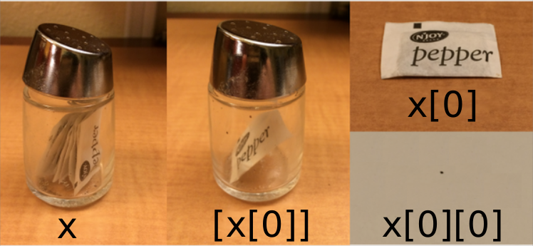
x = [['pepper', 'zucchini', 'onion'],
     ['cabbage', 'lettuce', 'garlic'],
     ['apple', 'pear', 'banana']]
Here is a visual example of how indexing a list of lists
xworks:
Using the previously declared list
x, these would be the results of the index operations shown in the image:print([x[0]])[['pepper', 'zucchini', 'onion']]print(x[0])['pepper', 'zucchini', 'onion']print(x[0][0])'pepper'Thanks to Hadley Wickham for the image above.
Heterogeneous Lists
Lists in Python can contain elements of different types. Example:
sample_ages = [10, 12.5, 'Unknown']
There are many ways to change the contents of lists besides assigning new values to individual elements:
odds.append(11)
print('odds after adding a value:', odds)
odds after adding a value: [1, 3, 5, 7, 11]
removed_element = odds.pop(0)
print('odds after removing the first element:', odds)
print('removed_element:', removed_element)
odds after removing the first element: [3, 5, 7, 11]
removed_element: 1
odds.reverse()
print('odds after reversing:', odds)
odds after reversing: [11, 7, 5, 3]
While modifying in place, it is useful to remember that Python treats lists in a slightly counter-intuitive way.
If we make a list and (attempt to) copy it then modify in place, we can cause all sorts of trouble:
odds = [1, 3, 5, 7]
primes = odds
primes.append(2)
print('primes:', primes)
print('odds:', odds)
primes: [1, 3, 5, 7, 2]
odds: [1, 3, 5, 7, 2]
This is because Python stores a list in memory, and then can use multiple names to refer to the
same list. If all we want to do is copy a (simple) list, we can use the list function, so we do
not modify a list we did not mean to:
odds = [1, 3, 5, 7]
primes = list(odds)
primes.append(2)
print('primes:', primes)
print('odds:', odds)
primes: [1, 3, 5, 7, 2]
odds: [1, 3, 5, 7]
This is different from how variables worked in lesson 1, and more similar to how a spreadsheet works.
Turn a String Into a List
Use a for-loop to convert the string “hello” into a list of letters:
["h", "e", "l", "l", "o"]Hint: You can create an empty list like this:
my_list = []Solution
my_list = []
for char in "hello":
    my_list.append(char)
print(my_list)
Subsets of lists and strings can be accessed by specifying ranges of values in brackets, similar to how we accessed ranges of positions in a NumPy array. This is commonly referred to as “slicing” the list/string.
binomial_name = "Drosophila melanogaster"
group = binomial_name[0:10]
print("group:", group)

species = binomial_name[11:23]
print("species:", species)

chromosomes = ["X", "Y", "2", "3", "4"]
autosomes = chromosomes[2:5]
print("autosomes:", autosomes)

last = chromosomes[-1]
print("last:", last)
group: Drosophila
species: melanogaster
autosomes: ["2", "3", "4"]
last: 4
Slicing From the End
Use slicing to access only the last four characters of a string or entries of a list.
string_for_slicing = "Observation date: 02-Feb-2013"
list_for_slicing = [["fluorine", "F"],
                    ["chlorine", "Cl"],
                    ["bromine", "Br"],
                    ["iodine", "I"],
                    ["astatine", "At"]]
"2013" [["chlorine", "Cl"], ["bromine", "Br"], ["iodine", "I"], ["astatine", "At"]]Would your solution work regardless of whether you knew beforehand the length of the string or list (e.g. if you wanted to apply the solution to a set of lists of different lengths)? If not, try to change your approach to make it more robust.
Hint: Remember that indices can be negative as well as positive
Solution
Use negative indices to count elements from the end of a container (such as list or string):
string_for_slicing[-4:]
list_for_slicing[-4:]
Non-Continuous Slices
So far we’ve seen how to use slicing to take single blocks of successive entries from a sequence. But what if we want to take a subset of entries that aren’t next to each other in the sequence?
You can achieve this by providing a third argument to the range within the brackets, called the step size. The example below shows how you can take every third entry in a list:
primes = [2, 3, 5, 7, 11, 13, 17, 19, 23, 29, 31, 37]
subset = primes[0:12:3]
print("subset", subset)
subset [2, 7, 17, 29]Notice that the slice taken begins with the first entry in the range, followed by entries taken at equally-spaced intervals (the steps) thereafter. If you wanted to begin the subset with the third entry, you would need to specify that as the starting point of the sliced range:
primes = [2, 3, 5, 7, 11, 13, 17, 19, 23, 29, 31, 37]
subset = primes[2:12:3]
print("subset", subset)
subset [5, 13, 23, 37]Use the step size argument to create a new string that contains only every other character in the string “In an octopus’s garden in the shade”
beatles = "In an octopus's garden in the shade"I notpssgre ntesaeSolution
To obtain every other character you need to provide a slice with the step size of 2:
beatles[0:35:2]You can also leave out the beginning and end of the slice to take the whole string and provide only the step argument to go every second element:
beatles[::2]
If you want to take a slice from the beginning of a sequence, you can omit the first index in the range:
date = "Monday 4 January 2016"
day = date[0:6]
print("Using 0 to begin range:", day)
day = date[:6]
print("Omitting beginning index:", day)
Using 0 to begin range: Monday
Omitting beginning index: Monday
And similarly, you can omit the ending index in the range to take a slice to the very end of the sequence:
months = ["jan", "feb", "mar", "apr", "may", "jun", "jul", "aug", "sep", "oct", "nov", "dec"]
sond = months[8:12]
print("With known last position:", sond)
sond = months[8:len(months)]
print("Using len() to get last entry:", sond)
sond = months[8:]
print("Omitting ending index:", sond)
With known last position: ["sep", "oct", "nov", "dec"]
Using len() to get last entry: ["sep", "oct", "nov", "dec"]
Omitting ending index: ["sep", "oct", "nov", "dec"]
Overloading
+usually means addition, but when used on strings or lists, it means “concatenate”. Given that, what do you think the multiplication operator*does on lists? In particular, what will be the output of the following code?counts = [2, 4, 6, 8, 10] repeats = counts * 2 print(repeats)
[2, 4, 6, 8, 10, 2, 4, 6, 8, 10][4, 8, 12, 16, 20][[2, 4, 6, 8, 10],[2, 4, 6, 8, 10]][2, 4, 6, 8, 10, 4, 8, 12, 16, 20]The technical term for this is operator overloading: a single operator, like
+or*, can do different things depending on what it’s applied to.Solution
The multiplication operator
*used on a list replicates elements of the list and concatenates them together:[2, 4, 6, 8, 10, 2, 4, 6, 8, 10]It’s equivalent to:
counts + counts
Analyzing Data from Multiple Files
We now have almost everything we need to process all our data files. The only thing that’s missing is a library with a rather unpleasant name:
import glob
The glob library contains a function, also called glob,
that finds files and directories whose names match a pattern.
We provide those patterns as strings:
the character * matches zero or more characters,
while ? matches any one character.
We can use this to get the names of all the CSV files in the current directory:
print(glob.glob('inflammation*.csv'))
['inflammation-05.csv', 'inflammation-11.csv', 'inflammation-12.csv', 'inflammation-08.csv',
'inflammation-03.csv', 'inflammation-06.csv', 'inflammation-09.csv', 'inflammation-07.csv',
'inflammation-10.csv', 'inflammation-02.csv', 'inflammation-04.csv', 'inflammation-01.csv']
As these examples show,
glob.glob’s result is a list of file and directory paths in arbitrary order.
This means we can loop over it
to do something with each filename in turn.
In our case,
the “something” we want to do is generate a set of plots for each file in our inflammation dataset.
If we want to start by analyzing just the first three files in alphabetical order, we can use the
sorted built-in function to generate a new sorted list from the glob.glob output:
import numpy
import matplotlib.pyplot

filenames = sorted(glob.glob('inflammation*.csv'))
filenames = filenames[0:3]
for f in filenames:
    print(f)

    data = numpy.loadtxt(fname=f, delimiter=',')

    fig = matplotlib.pyplot.figure(figsize=(10.0, 3.0))

    axes1 = fig.add_subplot(1, 3, 1)
    axes2 = fig.add_subplot(1, 3, 2)
    axes3 = fig.add_subplot(1, 3, 3)

    axes1.set_ylabel('average')
    axes1.plot(numpy.mean(data, axis=0))

    axes2.set_ylabel('max')
    axes2.plot(numpy.max(data, axis=0))

    axes3.set_ylabel('min')
    axes3.plot(numpy.min(data, axis=0))

    fig.tight_layout()
    matplotlib.pyplot.show()
inflammation-01.csv
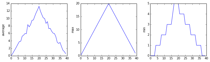
inflammation-02.csv
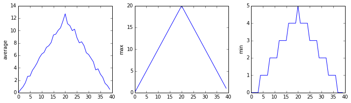
inflammation-03.csv

Sure enough, the maxima of the first two data sets show exactly the same ramp as the first, and their minima show the same staircase structure; a different situation has been revealed in the third dataset, where the maxima are a bit less regular, but the minima are consistently zero.
Plotting Differences
Plot the difference between the average of the first dataset and the average of the second dataset, i.e., the difference between the leftmost plot of the first two figures.
Solution
import glob
import numpy
import matplotlib.pyplot

filenames = sorted(glob.glob('inflammation*.csv'))

data0 = numpy.loadtxt(fname=filenames[0], delimiter=',')
data1 = numpy.loadtxt(fname=filenames[1], delimiter=',')

fig = matplotlib.pyplot.figure(figsize=(10.0, 3.0))

matplotlib.pyplot.ylabel('Difference in average')
matplotlib.pyplot.plot(numpy.mean(data0, axis=0) - numpy.mean(data1, axis=0))

fig.tight_layout()
matplotlib.pyplot.show()
Generate Composite Statistics
Use each of the files once to generate a dataset containing values averaged over all patients:
filenames = glob.glob('inflammation*.csv')
composite_data = numpy.zeros((60,40))
for f in filenames:
    # sum each new file's data into composite_data as it's read
    #
# and then divide the composite_data by number of samples
composite_data /= len(filenames)
Then use pyplot to generate average, max, and min for all patients.
Solution
import glob
import numpy
import matplotlib.pyplot

filenames = glob.glob('inflammation*.csv')
composite_data = numpy.zeros((60,40))

for f in filenames:
    data = numpy.loadtxt(fname = f, delimiter=',')
    composite_data += data

composite_data/=len(filenames)

fig = matplotlib.pyplot.figure(figsize=(10.0, 3.0))

axes1 = fig.add_subplot(1, 3, 1)
axes2 = fig.add_subplot(1, 3, 2)
axes3 = fig.add_subplot(1, 3, 3)

axes1.set_ylabel('average')
axes1.plot(numpy.mean(composite_data, axis=0))

axes2.set_ylabel('max')
axes2.plot(numpy.max(composite_data, axis=0))

axes3.set_ylabel('min')
axes3.plot(numpy.min(composite_data, axis=0))

fig.tight_layout()

matplotlib.pyplot.show()
Making Choices
In our last lesson, we discovered something suspicious was going on in our inflammation data by drawing some plots. How can we use Python to automatically recognize the different features we saw, and take a different action for each? In this lesson, we’ll learn how to write code that runs only when certain conditions are true.
Conditionals
We can ask Python to take different actions, depending on a condition, with an if statement:
num = 37
if num > 100:
    print('greater')
else:
    print('not greater')
print('done')
not greater
done
The second line of this code uses the keyword if to tell Python that we want to make a choice.
If the test that follows the if statement is true,
the body of the if
(i.e., the set of lines indented underneath it) is executed.
If the test is false,
the body of the else is executed instead.
Only one or the other is ever executed:

Conditional statements don’t have to include an else.
If there isn’t one,
Python simply does nothing if the test is false:
num = 53
print('before conditional...')
if num > 100:
    print(num,' is greater than 100')
print('...after conditional')
before conditional...
...after conditional
We can also chain several tests together using elif,
which is short for “else if”.
The following Python code uses elif to print the sign of a number.
num = -3

if num > 0:
    print(num, 'is positive')
elif num == 0:
    print(num, 'is zero')
else:
    print(num, 'is negative')
-3 is negative
Note that to test for equality we use a double equals sign ==
rather than a single equals sign = which is used to assign values.
We can also combine tests using and and or.
and is only true if both parts are true:
if (1 > 0) and (-1 > 0):
    print('both parts are true')
else:
    print('at least one part is false')
at least one part is false
while or is true if at least one part is true:
if (1 < 0) or (-1 < 0):
    print('at least one test is true')
at least one test is true
TrueandFalse
TrueandFalseare special words in Python calledbooleans, which represent truth values. A statement such as1 < 0returns the valueFalse, while-1 < 0returns the valueTrue.
Checking our Data
Now that we’ve seen how conditionals work,
we can use them to check for the suspicious features we saw in our inflammation data.
We are about to use functions provided by the numpy module again.
Therefore, if you’re working in a new Python session, make sure to load the
module with:
import numpy
From the first couple of plots, we saw that maximum daily inflammation exhibits a strange behavior and raises one unit a day. Wouldn’t it be a good idea to detect such behavior and report it as suspicious? Let’s do that! However, instead of checking every single day of the study, let’s merely check if maximum inflammation in the beginning (day 0) and in the middle (day 20) of the study are equal to the corresponding day numbers.
max_inflammation_0 = numpy.max(data, axis=0)[0]
max_inflammation_20 = numpy.max(data, axis=0)[20]

if max_inflammation_0 == 0 and max_inflammation_20 == 20:
    print('Suspicious looking maxima!')
We also saw a different problem in the third dataset;
the minima per day were all zero (looks like a healthy person snuck into our study).
We can also check for this with an elif condition:
elif numpy.sum(numpy.min(data, axis=0)) == 0:
    print('Minima add up to zero!')
And if neither of these conditions are true, we can use else to give the all-clear:
else:
    print('Seems OK!')
Let’s test that out:
data = numpy.loadtxt(fname='inflammation-01.csv', delimiter=',')

max_inflammation_0 = numpy.max(data, axis=0)[0]
max_inflammation_20 = numpy.max(data, axis=0)[20]

if max_inflammation_0 == 0 and max_inflammation_20 == 20:
    print('Suspicious looking maxima!')
elif numpy.sum(numpy.min(data, axis=0)) == 0:
    print('Minima add up to zero!')
else:
    print('Seems OK!')
Suspicious looking maxima!
data = numpy.loadtxt(fname='inflammation-03.csv', delimiter=',')

max_inflammation_0 = numpy.max(data, axis=0)[0]
max_inflammation_20 = numpy.max(data, axis=0)[20]

if max_inflammation_0 == 0 and max_inflammation_20 == 20:
    print('Suspicious looking maxima!')
elif numpy.sum(numpy.min(data, axis=0)) == 0:
    print('Minima add up to zero!')
else:
    print('Seems OK!')
Minima add up to zero!
In this way,
we have asked Python to do something different depending on the condition of our data.
Here we printed messages in all cases,
but we could also imagine not using the else catch-all
so that messages are only printed when something is wrong,
freeing us from having to manually examine every plot for features we’ve seen before.
How Many Paths?
Consider this code:
if 4 > 5:
    print('A')
elif 4 == 5:
    print('B')
elif 4 < 5:
    print('C')
Which of the following would be printed if you were to run this code? Why did you pick this answer?
- A
- B
- C
- B and C
Solution
C gets printed because the first two conditions,
4 > 5and4 == 5, are not true, but4 < 5is true.
What Is Truth?
TrueandFalsebooleans are not the only values in Python that are true and false. In fact, any value can be used in aniforelif. After reading and running the code below, explain what the rule is for which values are considered true and which are considered false.if '': print('empty string is true') if 'word': print('word is true') if []: print('empty list is true') if [1, 2, 3]: print('non-empty list is true') if 0: print('zero is true') if 1: print('one is true')
That’s Not Not What I Meant
Sometimes it is useful to check whether some condition is not true. The Boolean operator
notcan do this explicitly. After reading and running the code below, write someifstatements that usenotto test the rule that you formulated in the previous challenge.if not '': print('empty string is not true') if not 'word': print('word is not true') if not not True: print('not not True is true')
Close Enough
Write some conditions that print
Trueif the variableais within 10% of the variablebandFalseotherwise. Compare your implementation with your partner’s: do you get the same answer for all possible pairs of numbers?Solution 1
a = 5
b = 5.1

if abs(a - b) < 0.1 * abs(b):
    print('True')
else:
    print('False')
Solution 2
print(abs(a - b) < 0.1 * abs(b))This works because the Booleans
TrueandFalsehave string representations which can be printed.
In-Place Operators
Python (and most other languages in the C family) provides in-place operators that work like this:
x = 1 # original value x += 1 # add one to x, assigning result back to x x *= 3 # multiply x by 3 print(x)6Write some code that sums the positive and negative numbers in a list separately, using in-place operators. Do you think the result is more or less readable than writing the same without in-place operators?
Solution
positive_sum = 0
negative_sum = 0
test_list = [3, 4, 6, 1, -1, -5, 0, 7, -8]
for num in test_list:
    if num > 0:
        positive_sum += num
    elif num == 0:
        pass
    else:
        negative_sum += num
print(positive_sum, negative_sum)
Here
passmeans “don’t do anything”. In this particular case, it’s not actually needed, since ifnum == 0neither sum needs to change, but it illustrates the use ofelifandpass.
Sorting a List Into Buckets
In our
datafolder, large data sets are stored in files whose names start with “inflammation-“ and small data sets – in files whose names start with “small-“. We also have some other files that we do not care about at this point. We’d like to break all these files into three lists calledlarge_files,small_files, andother_files, respectively.Add code to the template below to do this. Note that the string method
startswithreturnsTrueif and only if the string it is called on starts with the string passed as an argument, that is:"String".startswith("Str")TrueBut
"String".startswith("str")FalseUse the following Python code as your starting point:
files = ['inflammation-01.csv',
         'myscript.py',
         'inflammation-02.csv',
         'small-01.csv',
         'small-02.csv']
large_files = []
small_files = []
other_files = []
Your solution should:
- loop over the names of the files
- figure out which group each filename belongs
- append the filename to that list
In the end the three lists should be:
large_files = ['inflammation-01.csv', 'inflammation-02.csv']
small_files = ['small-01.csv', 'small-02.csv']
other_files = ['myscript.py']
Solution
for file in files:
    if file.startswith('inflammation-'):
        large_files.append(file)
    elif file.startswith('small-'):
        small_files.append(file)
    else:
        other_files.append(file)

print('large_files:', large_files)
print('small_files:', small_files)
print('other_files:', other_files)
Counting Vowels
- Write a loop that counts the number of vowels in a character string.
- Test it on a few individual words and full sentences.
- Once you are done, compare your solution to your neighbor’s. Did you make the same decisions about how to handle the letter ‘y’ (which some people think is a vowel, and some do not)?
Solution
vowels = 'aeiouAEIOU'
sentence = 'Mary had a little lamb.'
count = 0
for char in sentence:
    if char in vowels:
        count += 1

print("The number of vowels in this string is " + str(count))
Creating Functions
At this point,
we’ve written code to draw some interesting features in our inflammation data,
loop over all our data files to quickly draw these plots for each of them,
and have Python make decisions based on what it sees in our data.
But, our code is getting pretty long and complicated;
what if we had thousands of datasets,
and didn’t want to generate a figure for every single one?
Commenting out the figure-drawing code is a nuisance.
Also, what if we want to use that code again,
on a different dataset or at a different point in our program?
Cutting and pasting it is going to make our code get very long and very repetitive,
very quickly.
We’d like a way to package our code so that it is easier to reuse,
and Python provides for this by letting us define things called ‘functions’ —
a shorthand way of re-executing longer pieces of code.
Let’s start by defining a function fahr_to_celsius that converts temperatures
from Fahrenheit to Celsius:
def fahr_to_celsius(temp):
    return ((temp - 32) * (5/9))

The function definition opens with the keyword def followed by the
name of the function (fahr_to_celsius) and a parenthesized list of parameter names (temp). The
body of the function — the
statements that are executed when it runs — is indented below the
definition line. The body concludes with a return keyword followed by the return value.
When we call the function, the values we pass to it are assigned to those variables so that we can use them inside the function. Inside the function, we use a return statement to send a result back to whoever asked for it.
Let’s try running our function.
fahr_to_celsius(32)
This command should call our function, using “32” as the input and return the function value.
In fact, calling our own function is no different from calling any other function:
print('freezing point of water:', fahr_to_celsius(32), 'C')
print('boiling point of water:', fahr_to_celsius(212), 'C')
freezing point of water: 0.0 C
boiling point of water: 100.0 C
We’ve successfully called the function that we defined, and we have access to the value that we returned.
Composing Functions
Now that we’ve seen how to turn Fahrenheit into Celsius, we can also write the function to turn Celsius into Kelvin:
def celsius_to_kelvin(temp_c):
    return temp_c + 273.15

print('freezing point of water in Kelvin:', celsius_to_kelvin(0.))
freezing point of water in Kelvin: 273.15
What about converting Fahrenheit to Kelvin? We could write out the formula, but we don’t need to. Instead, we can compose the two functions we have already created:
def fahr_to_kelvin(temp_f):
    temp_c = fahr_to_celsius(temp_f)
    temp_k = celsius_to_kelvin(temp_c)
    return temp_k

print('boiling point of water in Kelvin:', fahr_to_kelvin(212.0))
boiling point of water in Kelvin: 373.15
This is our first taste of how larger programs are built: we define basic operations, then combine them in ever-larger chunks to get the effect we want. Real-life functions will usually be larger than the ones shown here — typically half a dozen to a few dozen lines — but they shouldn’t ever be much longer than that, or the next person who reads it won’t be able to understand what’s going on.
Tidying up
Now that we know how to wrap bits of code up in functions,
we can make our inflammation analysis easier to read and easier to reuse.
First, let’s make an analyze function that generates our plots:
def analyze(filename):

    data = numpy.loadtxt(fname=filename, delimiter=',')

    fig = matplotlib.pyplot.figure(figsize=(10.0, 3.0))

    axes1 = fig.add_subplot(1, 3, 1)
    axes2 = fig.add_subplot(1, 3, 2)
    axes3 = fig.add_subplot(1, 3, 3)

    axes1.set_ylabel('average')
    axes1.plot(numpy.mean(data, axis=0))

    axes2.set_ylabel('max')
    axes2.plot(numpy.max(data, axis=0))

    axes3.set_ylabel('min')
    axes3.plot(numpy.min(data, axis=0))

    fig.tight_layout()
    matplotlib.pyplot.show()
and another function called detect_problems that checks for those systematics
we noticed:
def detect_problems(filename):

    data = numpy.loadtxt(fname=filename, delimiter=',')

    if numpy.max(data, axis=0)[0] == 0 and numpy.max(data, axis=0)[20] == 20:
        print('Suspicious looking maxima!')
    elif numpy.sum(numpy.min(data, axis=0)) == 0:
        print('Minima add up to zero!')
    else:
        print('Seems OK!')
Wait! Didn’t we forget to specify what both of these functions should return? Well, we didn’t.
In Python, functions are not required to include a return statement and can be used for
the sole purpose of grouping together pieces of code that conceptually do one thing. In such cases,
function names usually describe what they do, e.g. analyze, detect_problems.
Notice that rather than jumbling this code together in one giant for loop,
we can now read and reuse both ideas separately.
We can reproduce the previous analysis with a much simpler for loop:
filenames = sorted(glob.glob('inflammation*.csv'))

for f in filenames[:3]:
    print(f)
    analyze(f)
    detect_problems(f)
By giving our functions human-readable names,
we can more easily read and understand what is happening in the for loop.
Even better, if at some later date we want to use either of those pieces of code again,
we can do so in a single line.
Testing and Documenting
Once we start putting things in functions so that we can re-use them, we need to start testing that those functions are working correctly. To see how to do this, let’s write a function to offset a dataset so that it’s mean value shifts to a user-defined value:
def offset_mean(data, target_mean_value):
    return (data - numpy.mean(data)) + target_mean_value
We could test this on our actual data, but since we don’t know what the values ought to be, it will be hard to tell if the result was correct. Instead, let’s use NumPy to create a matrix of 0’s and then offset its values to have a mean value of 3:
z = numpy.zeros((2,2))
print(offset_mean(z, 3))
[[ 3.  3.]
 [ 3.  3.]]
That looks right,
so let’s try offset_mean on our real data:
data = numpy.loadtxt(fname='inflammation-01.csv', delimiter=',')
print(offset_mean(data, 0))
[[-6.14875 -6.14875 -5.14875 ..., -3.14875 -6.14875 -6.14875]
 [-6.14875 -5.14875 -4.14875 ..., -5.14875 -6.14875 -5.14875]
 [-6.14875 -5.14875 -5.14875 ..., -4.14875 -5.14875 -5.14875]
 ...,
 [-6.14875 -5.14875 -5.14875 ..., -5.14875 -5.14875 -5.14875]
 [-6.14875 -6.14875 -6.14875 ..., -6.14875 -4.14875 -6.14875]
 [-6.14875 -6.14875 -5.14875 ..., -5.14875 -5.14875 -6.14875]]
It’s hard to tell from the default output whether the result is correct, but there are a few simple tests that will reassure us:
print('original min, mean, and max are:', numpy.min(data), numpy.mean(data), numpy.max(data))
offset_data = offset_mean(data, 0)
print('min, mean, and max of offset data are:',
      numpy.min(offset_data),
      numpy.mean(offset_data),
      numpy.max(offset_data))
original min, mean, and max are: 0.0 6.14875 20.0
min, mean, and and max of offset data are: -6.14875 2.84217094304e-16 13.85125
That seems almost right: the original mean was about 6.1, so the lower bound from zero is now about -6.1. The mean of the offset data isn’t quite zero — we’ll explore why not in the challenges — but it’s pretty close. We can even go further and check that the standard deviation hasn’t changed:
print('std dev before and after:', numpy.std(data), numpy.std(offset_data))
std dev before and after: 4.61383319712 4.61383319712
Those values look the same, but we probably wouldn’t notice if they were different in the sixth decimal place. Let’s do this instead:
print('difference in standard deviations before and after:',
      numpy.std(data) - numpy.std(offset_data))
difference in standard deviations before and after: -3.5527136788e-15
Again, the difference is very small. It’s still possible that our function is wrong, but it seems unlikely enough that we should probably get back to doing our analysis. We have one more task first, though: we should write some documentation for our function to remind ourselves later what it’s for and how to use it.
The usual way to put documentation in software is to add comments like this:
# offset_mean(data, target_mean_value):
# return a new array containing the original data with its mean offset to match the desired value.
def offset_mean(data, target_mean_value):
    return (data - numpy.mean(data)) + target_mean_value
There’s a better way, though. If the first thing in a function is a string that isn’t assigned to a variable, that string is attached to the function as its documentation:
def offset_mean(data, target_mean_value):
    '''Return a new array containing the original data
       with its mean offset to match the desired value.'''
    return (data - numpy.mean(data)) + target_mean_value
This is better because we can now ask Python’s built-in help system to show us the documentation for the function:
help(offset_mean)
Help on function offset_mean in module __main__:

offset_mean(data, target_mean_value)
    Return a new array containing the original data with its mean offset to match the desired value.
A string like this is called a docstring. We don’t need to use triple quotes when we write one, but if we do, we can break the string across multiple lines:
def offset_mean(data, target_mean_value):
    '''Return a new array containing the original data
       with its mean offset to match the desired value.
    Example: offset_mean([1, 2, 3], 0) => [-1, 0, 1]'''
    return (data - numpy.mean(data)) + target_mean_value

help(offset_mean)
Help on function center in module __main__:

offset_mean(data, target_mean_value)
    Return a new array containing the original data with its mean offset to match the desired value.
    Example: offset_mean([1, 2, 3], 0) => [-1, 0, 1]
Defining Defaults
We have passed parameters to functions in two ways:
directly, as in type(data),
and by name, as in numpy.loadtxt(fname='something.csv', delimiter=',').
In fact,
we can pass the filename to loadtxt without the fname=:
numpy.loadtxt('inflammation-01.csv', delimiter=',')
array([[ 0.,  0.,  1., ...,  3.,  0.,  0.],
       [ 0.,  1.,  2., ...,  1.,  0.,  1.],
       [ 0.,  1.,  1., ...,  2.,  1.,  1.],
       ...,
       [ 0.,  1.,  1., ...,  1.,  1.,  1.],
       [ 0.,  0.,  0., ...,  0.,  2.,  0.],
       [ 0.,  0.,  1., ...,  1.,  1.,  0.]])
but we still need to say delimiter=:
numpy.loadtxt('inflammation-01.csv', ',')
Traceback (most recent call last):
  File "<stdin>", line 1, in <module>
  File "/Users/username/anaconda3/lib/python3.6/site-packages/numpy/lib/npyio.py", line 1041, in loa
dtxt
    dtype = np.dtype(dtype)
  File "/Users/username/anaconda3/lib/python3.6/site-packages/numpy/core/_internal.py", line 199, in
_commastring
    newitem = (dtype, eval(repeats))
  File "<string>", line 1
    ,
    ^
SyntaxError: unexpected EOF while parsing
To understand what’s going on,
and make our own functions easier to use,
let’s re-define our offset_mean function like this:
def offset_mean(data, target_mean_value=0.0):
    '''Return a new array containing the original data with its mean offset to match the
       desired value (0 by default).
    Example: offset_mean([1, 2, 3], 0) => [-1, 0, 1]'''
    return (data - numpy.mean(data)) + target_mean_value
The key change is that the second parameter is now written target_mean_value=0.0
instead of just target_mean_value.
If we call the function with two arguments,
it works as it did before:
test_data = numpy.zeros((2, 2))
print(offset_mean(test_data, 3))
[[ 3.  3.]
 [ 3.  3.]]
But we can also now call it with just one parameter,
in which case target_mean_value is automatically assigned
the default value of 0.0:
more_data = 5 + numpy.zeros((2, 2))
print('data before mean offset:')
print(more_data)
print('offset data:')
print(offset_mean(more_data))
data before mean offset:
[[ 5.  5.]
 [ 5.  5.]]
offset data:
[[ 0.  0.]
 [ 0.  0.]]
This is handy: if we usually want a function to work one way, but occasionally need it to do something else, we can allow people to pass a parameter when they need to but provide a default to make the normal case easier. The example below shows how Python matches values to parameters:
def display(a=1, b=2, c=3):
    print('a:', a, 'b:', b, 'c:', c)

print('no parameters:')
display()
print('one parameter:')
display(55)
print('two parameters:')
display(55, 66)
no parameters:
a: 1 b: 2 c: 3
one parameter:
a: 55 b: 2 c: 3
two parameters:
a: 55 b: 66 c: 3
As this example shows, parameters are matched up from left to right, and any that haven’t been given a value explicitly get their default value. We can override this behavior by naming the value as we pass it in:
print('only setting the value of c')
display(c=77)
only setting the value of c
a: 1 b: 2 c: 77
With that in hand,
let’s look at the help for numpy.loadtxt:
help(numpy.loadtxt)
Help on function loadtxt in module numpy.lib.npyio:

loadtxt(fname, dtype=<class 'float'>, comments='#', delimiter=None, converters=None, skiprows=0, use
cols=None, unpack=False, ndmin=0, encoding='bytes')
    Load data from a text file.

    Each row in the text file must have the same number of values.

    Parameters
    ----------
...
There’s a lot of information here, but the most important part is the first couple of lines:
loadtxt(fname, dtype=<class 'float'>, comments='#', delimiter=None, converters=None, skiprows=0, use
cols=None, unpack=False, ndmin=0, encoding='bytes')
This tells us that loadtxt has one parameter called fname that doesn’t have a default value,
and eight others that do.
If we call the function like this:
numpy.loadtxt('inflammation-01.csv', ',')
then the filename is assigned to fname (which is what we want),
but the delimiter string ',' is assigned to dtype rather than delimiter,
because dtype is the second parameter in the list. However ',' isn’t a known dtype so
our code produced an error message when we tried to run it.
When we call loadtxt we don’t have to provide fname= for the filename because it’s the
first item in the list, but if we want the ',' to be assigned to the variable delimiter,
we do have to provide delimiter= for the second parameter since delimiter is not
the second parameter in the list.
Readable functions
Consider these two functions:
def s(p):
    a = 0
    for v in p:
        a += v
    m = a / len(p)
    d = 0
    for v in p:
        d += (v - m) * (v - m)
    return numpy.sqrt(d / (len(p) - 1))

def std_dev(sample):
    sample_sum = 0
    for value in sample:
        sample_sum += value

    sample_mean = sample_sum / len(sample)

    sum_squared_devs = 0
    for value in sample:
        sum_squared_devs += (value - sample_mean) * (value - sample_mean)

    return numpy.sqrt(sum_squared_devs / (len(sample) - 1))
The functions s and std_dev are computationally equivalent (they
both calculate the sample standard deviation), but to a human reader,
they look very different. You probably found std_dev much easier to
read and understand than s.
As this example illustrates, both documentation and a programmer’s coding style combine to determine how easy it is for others to read and understand the programmer’s code. Choosing meaningful variable names and using blank spaces to break the code into logical “chunks” are helpful techniques for producing readable code. This is useful not only for sharing code with others, but also for the original programmer. If you need to revisit code that you wrote months ago and haven’t thought about since then, you will appreciate the value of readable code!
Combining Strings
“Adding” two strings produces their concatenation:
'a' + 'b'is'ab'. Write a function calledfencethat takes two parameters calledoriginalandwrapperand returns a new string that has the wrapper character at the beginning and end of the original. A call to your function should look like this:print(fence('name', '*'))*name*Solution
def fence(original, wrapper):
    return wrapper + original + wrapper
Return versus print
Note that
returnandreturnstatement, on the other hand, makes data visible to the program. Let’s have a look at the following function:def add(a, b): print(a + b)Question: What will we see if we execute the following commands?
A = add(7, 3)
print(A)
Solution
Python will first execute the function
addwitha = 7andb = 3, and, therefore, print10. However, because functionadddoes not have a line that starts withreturn(noreturn“statement”), it will, by default, return nothing which, in Python world, is calledNone. Therefore,Awill be assigned toNoneand the last line (print(A)) will printNone. As a result, we will see:10 None
Selecting Characters From Strings
If the variable
srefers to a string, thens[0]is the string’s first character ands[-1]is its last. Write a function calledouterthat returns a string made up of just the first and last characters of its input. A call to your function should look like this:print(outer('helium'))hmSolution
def outer(input_string):
    return input_string[0] + input_string[-1]
Rescaling an Array
Write a function
rescalethat takes an array as input and returns a corresponding array of values scaled to lie in the range 0.0 to 1.0. (Hint: IfLandHare the lowest and highest values in the original array, then the replacement for a valuevshould be(v-L) / (H-L).)Solution
def rescale(input_array):
    L = numpy.min(input_array)
    H = numpy.max(input_array)
    output_array = (input_array - L) / (H - L)
    return output_array
Testing and Documenting Your Function
Run the commands
help(numpy.arange)andhelp(numpy.linspace)to see how to use these functions to generate regularly-spaced values, then use those values to test yourrescalefunction. Once you’ve successfully tested your function, add a docstring that explains what it does.Solution
'''Takes an array as input, and returns a corresponding array scaled so
that 0 corresponds to the minimum and 1 to the maximum value of the input array.

Examples:
>>> rescale(numpy.arange(10.0))
array([ 0.        ,  0.11111111,  0.22222222,  0.33333333,  0.44444444,
       0.55555556,  0.66666667,  0.77777778,  0.88888889,  1.        ])
>>> rescale(numpy.linspace(0, 100, 5))
array([ 0.  ,  0.25,  0.5 ,  0.75,  1.  ])
'''
Defining Defaults
Rewrite the
rescalefunction so that it scales data to lie between0.0and1.0by default, but will allow the caller to specify lower and upper bounds if they want. Compare your implementation to your neighbor’s: do the two functions always behave the same way?Solution
def rescale(input_array, low_val=0.0, high_val=1.0):
    '''rescales input array values to lie between low_val and high_val'''
    L = numpy.min(input_array)
    H = numpy.max(input_array)
    intermed_array = (input_array - L) / (H - L)
    output_array = intermed_array * (high_val - low_val) + low_val
    return output_array
Variables Inside and Outside Functions
What does the following piece of code display when run — and why?
f = 0
k = 0

def f2k(f):
    k = ((f-32)*(5.0/9.0)) + 273.15
    return k

f2k(8)
f2k(41)
f2k(32)

print(k)
Solution
259.81666666666666
287.15
273.15
0
kis 0 because thekinside the functionf2kdoesn’t know about thekdefined outside the function.
Mixing Default and Non-Default Parameters
Given the following code:
def numbers(one, two=2, three, four=4):
    n = str(one) + str(two) + str(three) + str(four)
    return n

print(numbers(1, three=3))
what do you expect will be printed? What is actually printed? What rule do you think Python is following?
1234one2three41239SyntaxErrorGiven that, what does the following piece of code display when run?
def func(a, b=3, c=6):
    print('a: ', a, 'b: ', b, 'c:', c)

func(-1, 2)
a: b: 3 c: 6a: -1 b: 3 c: 6a: -1 b: 2 c: 6a: b: -1 c: 2Solution
Attempting to define the
numbersfunction results in4. SyntaxError. The defined parameterstwoandfourare given default values. Becauseoneandthreeare not given default values, they are required to be included as arguments when the function is called and must be placed before any parameters that have default values in the function definition.The given call to
funcdisplaysa: -1 b: 2 c: 6. -1 is assigned to the first parametera, 2 is assigned to the next parameterb, andcis not passed a value, so it uses its default value 6.
The Old Switcheroo
Consider this code:
a = 3
b = 7

def swap(a, b):
    temp = a
    a = b
    b = temp

swap(a, b)

print(a, b)
Which of the following would be printed if you were to run this code? Why did you pick this answer?
7 33 73 37 7Solution
3 7is the correct answer. Initially,ahas a value of 3 andbhas a value of 7. When theswapfunction is called, it creates local variables (also calledaandbin this case) and trades their values. The function does not return any values and does not alteraorboutside of its local copy. Therefore the original values ofaandbremain unchanged.
Readable Code
Revise a function you wrote for one of the previous exercises to try to make the code more readable. Then, collaborate with one of your neighbors to critique each other’s functions and discuss how your function implementations could be further improved to make them more readable.
Based on the tutorials by the The Carpentries.